Nearly a century before neural networks were first conceived, Ada Lovelace described an ambition to build a “calculus of the nervous system.” Although speculative analogies between brains and machines are as old as the philosophy of computation itself, it wasn’t until Ada’s teacher Charles Babbage proposed the Analytical engine that we conceived of “calculators” having humanlike cognitive capacities. Ada would not live to see her dream of building the engine come to fruitio n, as engineers of the time were unable to produce the complex circuitry her schematics required. Nevertheless, the idea was passed on to the next century when Alan Turing cited it as the inspiration for the Imitation Game, what soon came to be called the “Turing Test.” His ruminations into the extreme limits of computation incited the first boom of artificial intelligence, setting the stage for the first golden age of neural networks.
Birth and rebirth of neural nets
The recent resurgence of neural networks is a peculiar story. Intimately connected to the early days of AI, neural networks were first formalized in the late 1940s in the form of Turing’s B-type machines, drawing upon earlier research into neural plasticity by neuroscientists and cognitive psychologists studying the learning process in human beings. As the mechanics of brain development were being discovered, computer scientists experimented with idealized versions of action potential and neural backpropagation to simulate the process in machines.
Today, most scientists caution against taking this analogy too seriously, as neural networks are strictly designed for solving machine learning problems, rather than accurately depicting the brain, while a completely separate field called computational neuroscience has taken up the the challenge of faithfully modeling the brain. Nevertheless, the metaphor of the core unit of neural networks as a simplified biological neuron has stuck over the decades. The progression from biological neurons to artificial ones can be summarized by the following figures.
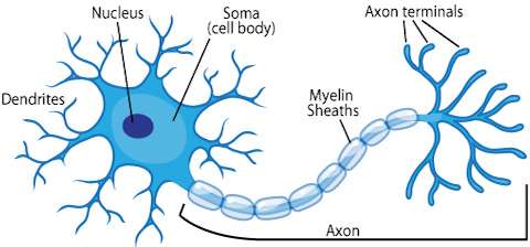
Source: ASU school of life sciences
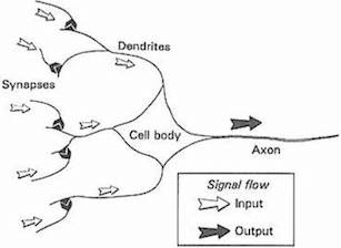
Source: Gurney, 1997. An Introduction to Neural Networks
Neural networks took a big step forward when Frank Rosenblatt devised the Perceptron in the late 1950s, a type of linear classifier that we saw in the last chapter. Publicly funded by the U.S. Navy, the Mark 1 perceptron was designed to perform image recognition from an array of photocells, potentiometers, and electrical motors. Its effectiveness at completing complex electrical circuits lead the New York Times in 1958 to predict that a machine would soon “walk, talk, see, write, reproduce itself and be conscious of its existence”.
The early hype would inspire science fiction writers for decades to come, but the excitement was far more tempered in the academic community. Marvin Minsky’s and Seymour Papert’s 1969 book, Perceptrons, demonstrated various-—even trivial—limitations, inadvertently leading to a decline of interest within both academia and the general public, who had mistakenly assumed computers would simply keep up with the breakneck pace of computational power. Even Turing himself said machines would possess human-level intelligence by the year 2000 – the year we had the Y2K scare.
Despite a number of quiet but significant improvements to neural networks in the 80s and 90s [1][2][3], they remained on the sidelines through the 2000s, with most commercial and industrial applications of machine learning favoring support vector machines and various other approaches. Starting in 2009 and especially ramping up from 2012, neural networks have once again become the dominant strain of ML algorithms. Their resurgence was largely brought about by the emergence of convolutional and recurrent neural networks, which have surpassed (sometimes dramatically so) previous state-of-the-art methods for key problems in the audiovisual domain. But more interestingly, they have a number of new applications and properties not seen before, especially of a kind that has piqued the interest of artists and others from outside the AI field proper. This book will look more closely at convolutional neural networks in particular several chapters from now.
Although many learning algorithms have been proposed over the years, we will mostly focus our attention on neural networks because:
- They have a surprisingly simple and intuitive formulation.
- Deep neural networks are the current state-of-the-art in several important machine learning tasks, the ones most relevant to this book.
- Most of the recent creative uses of machine learning have been made with neural networks.
From linear classifiers to neurons
Recall from the previous chapter that the input to a 2d linear classifier or regressor has the form:
\[\begin{eqnarray} f(x_1, x_2) = b + w_1 x_1 + w_2 x_2 \end{eqnarray}\]More generally, in any number of dimensions, it can be expressed as
\[\begin{eqnarray} f(X) = b + \sum_i w_i x_i \end{eqnarray}\]In the case of regression, \(f(X)\) gives us our predicted output, given the input vector \(X\). In the case of classification, our predicted class is given by
\[\begin{eqnarray} \mbox{classification} & = & \left\{ \begin{array}{ll} 1 & \mbox{if } f(X) \gt 0 \\ 0 & \mbox{if } f(X) \leq 0 \end{array} \right. \tag{1}\end{eqnarray}\]Each weight, \(w_i\), can be interpreted as signifying the relative influence of the input that it’s multiplied by, \(x_i\). The \(b\) term in the equation is often called the bias, because it controls how predisposed the neuron is to firing a 1 or 0, irrespective of the weights. A high bias makes the neuron require a larger input to output a 1, and a lower one makes it easier.
We can get from this formula to a full-fledged neural network by introducing two innovations. The first is the addition of an activation function, which turns our linear discriminator into what’s called a neuron, or a “unit” (to dissociate them from the brain analogy). The second innovation is an architecture of neurons which are connected sequentially in layers. We will introduce these innovations in that order.
Activation function
In both artificial and biological neural networks, a neuron does not just output the bare input it receives. Instead, there is one more step, called an activation function, analagous to the rate of action potential firing in the brain. The activation function takes the same weighted sum input from before, \(z = b + \sum_i w_i x_i\), and then transforms it once more before finally outputting it.
Many activation functions have been proposed, but for now we will describe two in detail: sigmoid and ReLU.
Historically, the sigmoid function is the oldest and most popular activation function. It is defined as:
\[\sigma(x) = \frac{1}{1 + e^{-x}}\]\(e\) denotes the exponential constant, roughly equal to 2.71828. A neuron which uses a sigmoid as its activation function is called a sigmoid neuron. We first set the variable \(z\) to our original weighted sum input, and then pass that through the sigmoid function.
\[z = b + \sum_i w_i x_i \\ \sigma(z) = \frac{1}{1 + e^{-z}}\]At first, this equation may seem complicated and arbitrary, but it actually has a very simple shape, which we can see if we plot the value of \(\sigma(z)\) as a function of the input \(z\).
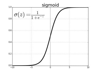
We can see that \(\sigma(z)\) acts as a sort of “squashing” function, condensing our previously unbounded output to the range 0 to 1. In the center, where \(z = 0\), \(\sigma(0) = 1/(1+e^{0}) = 1/2\). For large negative values of \(z\), the \(e^{-z}\) term in the denominator grows exponentially, and \(\sigma(z)\) approaches 0. Conversely, large positive values of \(z\) shrink \(e^{-z}\) to 0, so \(\sigma(z)\) approaches 1.
The sigmoid function is continuously differentiable, and its derivative, conveniently, is \(\sigma^\prime(z) = \sigma(z) (1-\sigma(z))\). This is important because we have to use calculus to train neural networks, but don’t worry about that for now.
Sigmoid neurons were the basis of most neural networks for decades, but in recent years, they have fallen out of favor. The reason for this will be explained in more detail later, but in short, they make neural networks that have many layers difficult to train due to the vanishing gradient problem. Instead, most have shifted to using another type of activation function, the rectified linear unit, or ReLU for short. Despite its obtuse name, it is simply defined as \(R(z) = max(0, z)\).
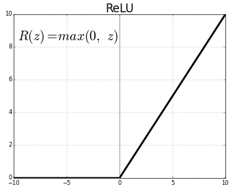
In other words, ReLUs let all positive values pass through unchanged, but just sets any negative value to 0. Although newer activation functions are gaining traction, most deep neural networks these days use ReLU or one of its closely related variants.
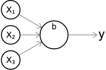
Regardless of which activation function is used, we can visualize a single neuron with this standard diagram, giving us a nice intuitive visual representation of a neuron’s behavior.
The above diagram shows a neuron with three inputs, and outputs a single value \(y\). As before, we first compute the weighted sum of its inputs, then pass it through an activation function \(\sigma\).
\[z = b + w_1 x_1 + w_2 x_2 + w_3 x_3 \\ y = \sigma(z)\]You may be wondering what the purpose of an activation function is, and why it is preferred to simply outputting the weighted sum, as we do with the linear classifier from the last chapter. The reason is that the weighted sum, \(z\), is linear with respect to its inputs, i.e. it has a flat dependence on each of the inputs. In contrast, non-linear activation functions greatly expand our capacity to model curved or otherwise non-trivial functions. This will become clearer in the next section.
Layers
Now that we have described neurons, we can now define neural networks. A neural network is composed of a series of layers of neurons, such that all the neurons in each layer connect to the neurons in the next layer.
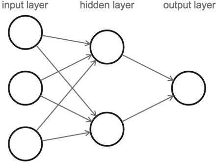
Note that when we count the number of layers in a neural network, we only count the layers with connections flowing into them (omitting our first, or input layer). So the above figure is of a 2-layer neural network with 1 hidden layer. It contains 3 input neurons, 2 neurons in its hidden layer, and 1 output neuron.
Our computation starts with the input layer on the left, from which we pass the values to the hidden layer, and then in turn, the hidden layer will send its output values to the last layer, which contains our final value.
Note that it may look like the three input neurons send out multiple values because each of them are connected to both of the neurons in the hidden layer. But really there is still only one output value per neuron, it just gets copied along each of its output connections. Neurons always output one value, no matter how many subsequent neurons it sends it to.
Regression
The process of a neural network sending an initial input forward through its layers to the output is called forward propagation or a forward pass and any neural network which works this way is called a feedforward neural network. As we shall soon see, there are some neural networks which allow data to flow in circles, but let’s not get ahead of ourselves yet…
Let’s demonstrate a forward pass with this interactive demo. Click the ‘Next’ button in the top-right corner to proceed.
More layers, more expressiveness
Why are hidden layers useful? The reason is that if we have no hidden layers and map directly from inputs to output, each input’s contribution on the output is independent of the other inputs. In real-world problems, input variables tend to be highly interdependent and they affect the output in combinatorially intricate ways. The hidden layer neurons allow us to capture subtle interactions among our inputs which affect the final output downstream. Another way to interpret this is that the hidden layers represent higher-level “features” or attributes of our data. Each of the neurons in the hidden layer weigh the inputs differently, learning some different intermediary characteristic of the data, and our output neuron is then a function of these instead of the raw inputs. By including more than one hidden layer, we give the network an opportunity to learn multiple levels of abstraction of the original input data before arriving at a final output. This notion of high-level features will become more concrete in the next chapter when we look closely at the hidden layers.
Recall also that activation functions expand our capacity to capture non-linear relationships between inputs and outputs. By chaining multiple non-linear transformations together through layers, this dramatically increases the flexibility and expressiveness of neural networks. The proof of this is complex and beyond the scope of this book, but it can even be shown that any 2-layer neural network with a non-linear activation function (including sigmoid or ReLU) and enough hidden units is a universal function approximator, that is it’s theoretically capable of expressing any arbitrary input-to-output mapping. This property is what makes neural networks so powerful.
Classification
What about classification? In the previous chapter, we introduced binary classification by simply thresholding the output at 0; If our output was positive, we’d classify positively, and if it was negative, we’d classify negatively. For neural networks, it would be reasonable to adapt this approach for the final neuron, and classify positively if the output neuron scores above some threshold. For example, we can threshold at 0.5 for sigmoid neurons which are always positive.
But what if we have multiple classes? One option might be to create intervals in the output neuron which correspond to each class, but this would be problematic for reasons that we will learn about when we look at how neural networks are trained. Instead, neural networks are adapted for classification by having one output neuron for each class. We do a forward pass and our prediction is the class corresponding to the neuron which received the highest value. Let’s have a look at an example.
Classification of handwritten digits
Let’s now tackle a real world example of classification using neural networks, the task of recognizing and labeling images of handwritten digits. We are going to use the MNIST dataset, which contains 60,000 labeled images of handwritten digits sized 28x28 pixels, whose classification accuracy serves as a common benchmark in machine learning research. Below is a random sample of images found in the dataset.
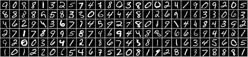
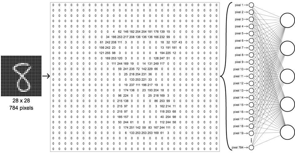
The way we setup a neural network to classify these images is by having the raw pixel values be our first layer inputs, and having 10 output classes, one for each of our digit classes from 0 to 9. Since they are grayscale images, each pixel has a brightness value between 0 (black) and 255 (white). All the MNIST images are 28x28, so they contain 784 pixels. We can unroll these into a single array of inputs, like in the following figure.
The important thing to realize is that although this network seems a lot more imposing than our simple 3x2x1 network in the previous chapter, it works exactly as before, just with many more neurons. Each neuron in the first hidden layer receives all the inputs from the first layer. For the output layer, we’ll now have ten neurons rather than just one, with full connections between it and the hidden layer, as before. Each of the ten output neurons is assigned to one class label; the first one is for the digit 0, the second for 1, and so on.
After the neural network has been trained – something we’ll talk about in more detail in a future chapter – we can predict the digit associated with unknown samples by running them through the same network and observing the output values. The predicted digit is that whose output neuron has the highest value at the end. The following demo shows this in action; click “next” to flip through more predictions.
Further reading
Next chapter
In the next chapter, looking inside neural networks, we will analyze the internal states of neural networks more closely, building up intuitions on what sorts of information they capture, as well as pointing out the flaws of basic neural nets, building up motivation for introducing more complex features such as convolutional layers to be explored in later chapters.