In the previous chapter, we saw how a neural network can be trained to classify handwritten digits with a respectable accuracy of around 90%. In this chapter, we are going to evaluate its performance a little more carefully, as well as examine its internal state to develop a few intuitions about what’s really going on. Later in this chapter, we are going to break our neural network altogether by attempting to train it on a more complicated dataset of objects like dogs, automobiles, and ships, to try to anticipate what kinds of innovations will be necessary to take it to the next level.
Visualizing weights
Let’s take a network trained to classify MNIST handwritten digits, except unlike in the last chapter, we will map directly from the input layer to the output layer with no hidden layers in between. Thus our network looks like this.
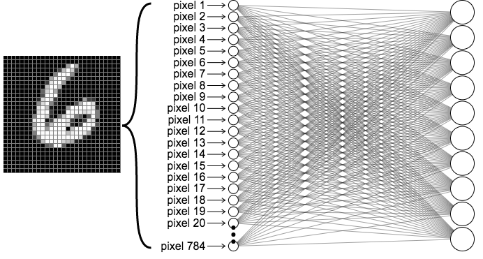
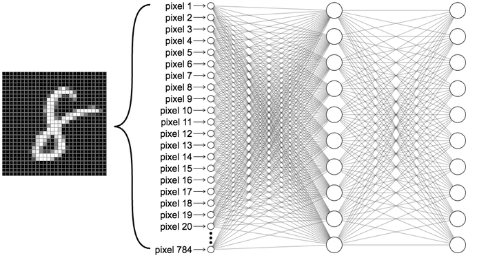
Recall that when we input an image into our neural net, we visualize the network diagram by “unrolling” the pixels into a single column of neurons, as shown in the below figure on the left. Let’s focus on just the connections plugged into the first output neuron, which we will label \(z\), and label each of the input neurons and their corresponding weights as \(x_i\) and \(w_i\).
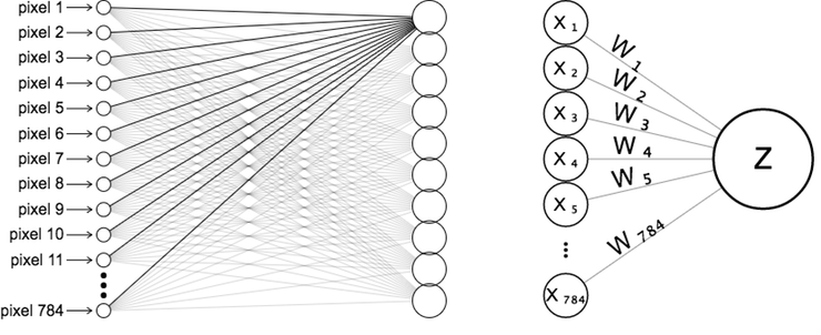
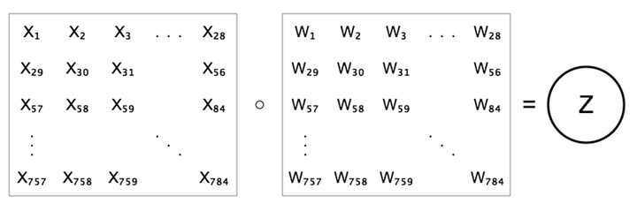
Rather than unrolling the pixels though, let’s instead view the weights as a 28x28 grid where the weights are arranged exactly like their corresponding pixels. The representation on the above right looks different from the one in the below figure, but they are expressing the same equation, namely \(z=b+\sum{w x}\).
Now let’s take a trained neural network with this architecture, and visualize the learned weights feeding into the first output neuron, which is the one responsible for classifying the digit 0. We color-code them so the lowest weight is black, and the highest is white.
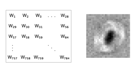
Squint your eyes a bit… does it look a bit like a blurry 0? The reason why it appears this way becomes more clear if we think about what that neuron is doing. Because it is “responsible” for classifying 0s, its goal is to output a high value for 0s and a low value for non-0s. It can get high outputs for 0s by having large weights aligned to pixels which tend to usually be high in images of 0s. Simultaneously, it can obtain relatively low outputs for non-0s by having small weights aligned to pixels which tend to be high in images of non-0s and low in images of 0s. The relatively black center of the weights image comes from the fact that images of 0s tend to be off here (the hole inside the 0), but are usually higher for the other digits.
Let’s look at the weights learned for all 10 of the output neurons. As suspected, they all look like somewhat blurry versions of our ten digits. They appear almost as though we averaged many images belonging to each digit class.
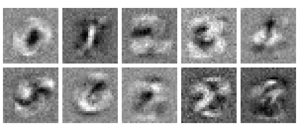
Suppose we receive an input from an image of a 2. We can anticipate that the neuron responsible for classifying 2s should have a high value because its weights are such that high weights tend to align with pixels tending to be high in 2s. For other neurons, some of the weights will also line up with high-valued pixels, making their scores somewhat higher as well. However, there is much less overlap, and many of the high-valued pixels in those images will be negated by low weights in other neurons. The activation function does not change this, because it is monotonic with respect to the input, that is, the higher the input, the higher the output.
We can interpret these weights as forming templates of the output classes. This is really fascinating because we never told our network anything in advance about what these digits are or what they mean, yet they came to resemble those object classes anyway. This is a hint of what’s really special about the internals of neural networks: they form representations of the objects they are trained on, and it turns out these representations can be useful for much more than simple classification or prediction. We will take this representational capacity to the next level when we begin to study convolutional neural networks but let’s not get ahead of ourselves yet…
This raises many more questions than it provides answers, such as what happens to the weights when we add hidden layers? As we will soon see, the answer to this will build upon what we saw in the previous section in an intuitive way. But before we get to that, it will help to examine the performance of our neural network, and in particular, consider what sorts of mistakes it tends to make.
0op5, 1 d14 17 2ga1n
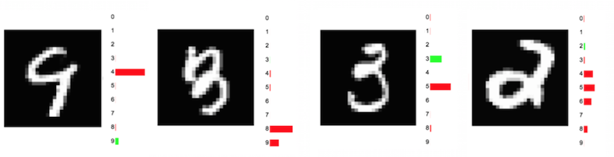
Occasionally, our network will make mistakes that we can sympathize with. To my eye, it’s not obvious that the first digit below is 9. One could easily mistake it for a 4, as our network did. Similarly, one could understand why the second digit, a 3, was misclassified by the network as an 8. The mistakes on the third and fourth digits below are more glaring. Almost any person would immediately recognize them as a 3 and a 2, respectively, yet our machine misinterpreted the first as a 5, and is nearly clueless on the second.
Let’s look more closely at the performance of the last neural network of the previous chapter, which achieved 90% accuracy on MNIST digits. One way we can do this is by looking at a confusion matrix, a table which breaks down our predictions into a table. In the following confusion matrix, the 10 rows correspond to the actual labels of the MNIST dataset, and the columns represent the predicted labels. For example, the cell at the 4th row and 6th column shows us that there were 71 instances in which an actual 3 was mislabeled by our neural network as a 5. The green diagonal of our confusion matrix shows us the quantities of correct predictions, whereas every other cell shows mistakes.
Hover your mouse over each cell to get a sampling of the top instances from each cell, ordered by the network’s confidence (probability) for the prediction.
We can also get some nice insights by plotting the top sample for each cell of the confusion matrix, as seen below.
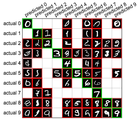
This gives us an impression of how the network learns to make certain kinds of predictions. Looking at first two columns, we see that our network appears to be looking for big loops to predict 0s, and thin lines to predict 1s, mistaking other digits if they happen to have those features.
Breaking our neural network
So far we’ve looked only at neural networks trained to identify handwritten digits. This gives us many insights but is a very easy choice of dataset, giving us many advantages; We have only ten classes, which are very well-defined and have relatively little internal variance among them. In most real-world scenarios, we are trying to classify images under much less ideal circumstances. Let’s look at the performance of the same neural network on another dataset, CIFAR-10, a labeled set of 60,000 32x32 color images belonging to ten classes: airplanes, automobiles, birds, cats, deer, dogs, frogs, horses, ships, and trucks. The following is a random sample of images from CIFAR-10.
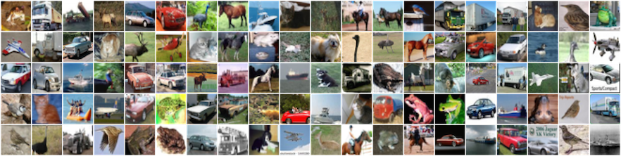
Right away, it’s clear we must contend with the fact that these image classes differ in ways that we haven’t dealt with yet. For example, cats can be facing different directions, have different colors and fur patterns, be outstretched or curled up, and many other variations we don’t encounter with handwritten digits. Photos of cats will also be cluttered with other objects, further complicating the problem.
Sure enough, if we train a 2-layer neural network on these images, our accuracy reaches only 37%. That’s still much better than taking random guesses (which would get us a 10% accuracy) but it’s far short of the 90% our MNIST classifier achieves. When we start convolutional neural networks, we’ll improve greatly on those numbers, for both MNIST and CIFAR-10. For now, we can get a more precise sense about the shortcomings of ordinary neural networks by inspecting their weights.
Let’s repeat the earlier experiment of observing the weights of a 1-layer neural network with no hidden layer, except this time training on images from CIFAR-10. The weights appear below.
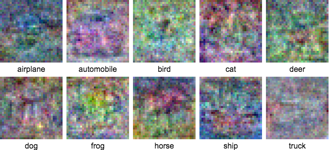
Compared to the MNIST weights, these have fewer obvious features and far less definition to them. Certain details do make intuitive sense, e.g. airplanes and ships are mostly blue on the outer edges of the images, reflecting the tendency for those images to have blue skies or waters around them. Because the weights image for a particular class does correlate to an average of images belonging to that class, we can expect blobby average colors to come out, as before. But because the CIFAR classes are much less internally consistent, the well-defined “templates” we saw with MNIST are far less evident.
Let’s take a look at the confusion matrix associated with this CIFAR-10 classifier.
Not surprisingly, its performance is very poor, reaching only 37% accuracy. Clearly, our simple 1-layer neural network is not capable of capturing the complexity of this dataset. One way we can improve its performance somewhat is by introducing a hidden layer. The next section will analyze the effects of doing that.
Adding hidden layers
So far, we’ve focused on 1-layer neural networks where the inputs connect directly to the outputs. How do hidden layers affect our neural network? To see, let’s try inserting a middle layer of ten neurons into our MNIST network. So now, our neural network for classifying handwritten digits looks like the following.
Our simple template metaphor in the 1-layer network above doesn’t apply to this case, because we no longer have the 784 input pixels connecting directly to the output classes. In some sense, you could say that we had “forced” our original 1-layer network to learn those templates because each of the weights connected directly into a single class label, and thus only affected that class. But in the more complicated network that we have introduced now, the weights in the hidden layer affect all ten of the neurons in the output layer. So how should we expect those weights to look now?
To understand what’s going on, we will visualize the weights in the first layer, as before, but we’ll also look carefully at how their activations are then combined in the second layer to obtain class scores. Recall that an image will generate a high activation in a particular neuron in the first layer if the image is largely sympathetic to that filter. So the ten neurons in the hidden layer reflect the presence of those ten features in the original image. In the output layer, a single neuron, corresponding to a class label, is a weighted combination of those previous ten hidden activations. Let’s look at them below.
Let’s start with the first layer weights, visualized at the top. They don’t look like the image class templates anymore, but rather more unfamiliar. Some look like pseudo-digits, and others appear to be components of digits: half loops, diagonal lines, holes, and so on.
The rows below the filter images correspond to our output neurons, one for each image class. The bars signify the weights associated to each of the ten filters’ activations from the hidden layer. For example, the 0 class appears to favor first layer filters which are high along the outer rim (where a zero digit tends to appear). It disfavors filters where pixels in the middle are high (where the hole in zeros is usually found). The 1 class is almost the opposite of this, preferring filters which are strong in the middle, where you might expect the vertical stroke of a 1 to be drawn.
The advantage of this approach is flexibility. For each class, there is a wider array of input patterns that stimulate the corresponding output neuron. Each class can be triggered by the presence of several abstract features from the previous hidden layer, or some combination of them. Essentially, we can learn different kinds of zeros, different kinds of ones, and so on for each class. This will usually–but not always–improve the performance of the network for most tasks.
Features and representations
Let’s generalize some of what we’ve learned in this chapter. In single-layer and multi-layer neural networks, each layer has a similar function; it transforms data from the previous layer into a “higher-level” representation of that data. By “higher-level,” we mean that it contains a compact and more salient representation of that data, in the way that a summary is a “high-level” representation of a book. For example, in the 2-layer network above, we mapped the “low-level” pixels into “higher-level” features found in digits (strokes, loops, etc) in the first layer, and then mapped those high-level features into an even higher-level representation in the next layer, that of the actual digits. This notion of transforming data into smaller but more meaningful information is at the heart of machine learning, and a primary capability of neural networks.
By adding a hidden layer into a neural network, we give it a chance to learn features at multiple levels of abstraction. This gives us a rich representation of the data, in which we have low-level features in the early layers, and high-level features in the later layers which are composed of the previous layers’ features.
As we saw, hidden layers can improve accuracy, but only to a limited extent. Adding more and more layers stops improving accuracy quickly, and comes at a computational cost – we can’t simply ask our neural network to memorize every possible version of an image class through its hidden layers. It turns out there is a better way, using convolutional neural networks, which will be covered in a later chapter.
Further reading
Next chapter
In the next chapter, we will learn about a critical topic that we’ve glossed over up until now, how neural networks are trained: the process by which neural nets are constructed and trained on data, using a technique called gradient descent via backpropagation. We will build up our knowledge starting from simple linear regression, and working our way up through examples, and elaborating on the various aspects of training which researchers must deal with.