Convolutional neural networks – CNNs or convnets for short – are at the heart of deep learning, emerging in recent years as the most prominent strain of neural networks in research. They have revolutionized computer vision, achieving state-of-the-art results in many fundamental tasks, as well as making strong progress in natural language processing, computer audition, reinforcement learning, and many other areas. Convnets have been widely deployed by tech companies for many of the new services and features we see today. They have numerous and diverse applications, including:
- detecting and labeling objects, locations, and people in images
- converting speech into text and synthesizing audio of natural sounds
- describing images and videos with natural language
- tracking roads and navigating around obstacles in autonomous vehicles
- analyzing videogame screens to guide autonomous agents playing them
- “hallucinating” images, sounds, and text with generative models
Although convnets have been around since the 1980s (at least in their current form) and have their roots in earlier neuroscience research, they’ve only recently achieved fame in the wider scientific community for a series of remarkable successes in important scientific problems across multiple domains. They extend neural networks primarily by introducing a new kind of layer, designed to improve the network’s ability to cope with variations in position, scale, and viewpoint. Additionally, they have become increasingly deep, containing upwards of dozens or even hundreds of layers, forming hierarchically compositional models of images, sounds, as well as game boards and other spatial data structures.
Because of their success at vision-oriented tasks, they have been adopted by creative technologists and interaction designers, allowing their installations not only to detect movement, but to actively identify, describe, and track objects in physical spaces. They were also the driving force behind Deepdream and style transfer, the neural applications which first caught the attention of new media artists.
The next few chapters will focus on convnets and their applications, with this one formulating them and how they work, the next one describing their properties, and subsequent chapters focusing on their creative and artistic applications.
Weaknesses of ordinary neural nets
To understand the innovations convnets offer, it helps to first review the weaknesses of ordinary neural networks, which are covered in more detail in the prior chapter, Looking inside neural nets.
Recall that in a trained one-layer ordinary neural network, the weights between the input pixels and the output neurons end up looking like templates for each output class. This is because they are constrained to capture all the information about each class in a single layer. Each of these templates looks like an average of samples belonging to that class.
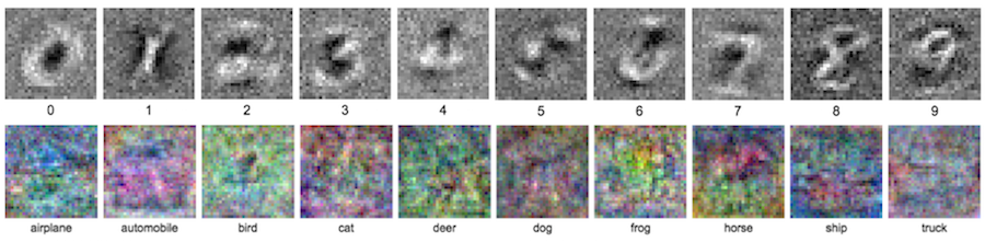
In the case of the MNIST dataset, we see that the templates are relatively discernible and thus effective, but for CIFAR-10, they are much more difficult to recognize. The reason is that the image categories in CIFAR-10 have a great deal more internal variation than MNIST. Images of dogs may contain dogs which are curled up or outstretched, have different fur colors, be cluttered with other objects, and various other distortions. Forced to learn all of these variations in one layer, our network can do no better than form a very weak average over all dog pictures, and which will fail to accurately recognize unseen ones on a consistent basis.
We can combat this by creating hidden layers, giving our network the capacity to form a hierarchy of discovered features. For example, suppose we make a 2-layer neural network for classifying MNIST, which contains a hidden layer containing 10 neurons and a final output layer also containing 10 neurons for our digits (as before). We train the network and extract the weights. In the following figure, we visualize the first layer weights using the same method as before, and we also visualize, as bar graphs, the second layer weights which connect our 10 hidden neurons to our 10 output neurons (we display just the first two classes for brevity).
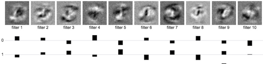
The first-layer weights can still be visualized in the same way as before, but instead of looking like the digits themselves, they appear to be fragments of them, or perhaps more general shapes and patterns that can be found in all of the digits to varying degrees. The first row bar graph depicts the relative contribution of each of the hidden layer neurons to the output neuron which classifies 0-digits. It appears to favor those first-layer neurons which have outer rings and it disfavors those with high weights in the middle. The second row is the same visualization for the output 1-neuron, which prefers those hidden neurons which show strong activity for images whose middle pixels are high. Thus we can see that the network can learn features that are more general to handwritten digits in the first layer and may be present in some digits but not in others. For example, outer loops or rings are useful for 8 and 0 but not 1 or 7; a diagonal stroke through the middle is useful for 7 and 2 but not 5 or 0, a quick inflection in the top-right is useful for 2, 7, and 9, but not for 5 or 6.
As a related example in the case of CIFAR-10, we saw earlier that many of the pictures of horses are of left-facing and right-facing horses, making the above template faintly resemble a two-headed horse. If we create a hidden layer, our network could potentially form learn a “right-facing horse” and “left-facing horse” template in the hidden layer, and the output neuron for horse could have strong weights for each of them. This isn’t a particularly elegant improvement, but as we scale it up, we see how such a strategy gives our network more flexibility. In early layers it can learn more specific and general features, which can then be combined in later layers.
Despite these improvements, it’s still impractical for the network to be able to memorize the nearly endless set of permutations which would fully characterize a dataset of diverse images. In order to capture that much information, we’d need too many neurons for what we can practically afford to store or train. The advantage of convnets is that they will allow us to capture these permutations in a more efficient way.
Compositionality
How can we encode variations among many classes of images efficiently? We can get some intuition to this question by considering an example.
Suppose I show you a picture of a car that you’ve never seen before. Chances are you’ll be able to identify it as a car by observing that it is a permutation of the various properties of cars. In other words, the picture contains some combination of the parts that make up most cars, including a windshield, wheels, doors, and exhaust pipe. By recognizing each of the smaller parts and adding them up, you realize that this picture is of a car, despite having never encountered this precise combination of those parts.
A convnet tries to do something similar: learn the individual parts of objects and store them in individual neurons, then add them up to recognize the larger object. This approach is advantageous for two reasons. One is that we can capture a greater variety of a particular object within a smaller number of neurons. For example, suppose we memorize 10 templates for different types of wheels, 10 templates for doors, and 10 for windshields. We thus capture $10 * 10 * 10 = 1000$ different cars for the price of only 30 templates. This is much more efficient than keeping around 1000 separate templates for cars, which contain much redundancy within them. But even better, we can reuse the smaller templates for different object classes. Wagons also have wheels. Houses also have doors. Ships also have windshields. We can construct a set of many more object classes as various combinations of these smaller parts, and do so very efficiently.
Antecedents and history of convnets
Before formally showing how convnets detect these kinds of features, let’s take a look at some of the important antecedents to them, to understand the evolution of our methods for combating the problems we described earlier.
Experiments of Hubel & Wiesel (1960s)
During the 1960s, neurophysiologists David Hubel and Torsten Wiesel conducted a series of experiments to investigate the properties of the visual cortices of animals. In one of the most notable experiments, they measured the electrical responses from a cat’s brain while stimulating it with simple patterns on a television screen. What they found was that neurons in the early visual cortex are organized in a hierarchical fashion, where the first cells connected to the cat’s retinas are responsible for detecting simple patterns like edges and bars, followed by later layers responding to more complex patterns by combining the earlier neuronal activities.
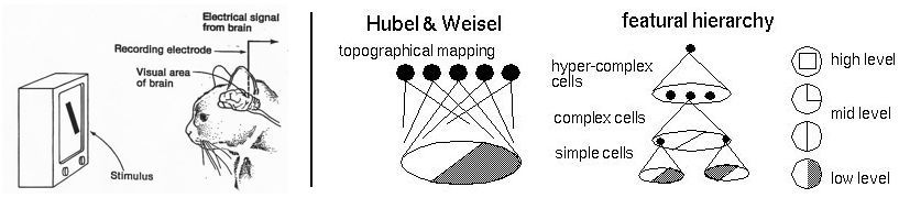
Later experiments on macaque monkeys revealed similar structures, and continued to refine an emerging understanding of mammalian visual processing. Their experiments would provide an early inspiration to artificial intelligence researchers seeking to construct well-defined computational frameworks for computer vision.
Fukushima’s Neocognitron (1982)
Hubel and Wiesel’s experiments were directly cited as inspiration by Kunihiko Fukushima in devising the Neocognitron, a neural network which attempted to mimic these hierarchical and compositional properties of the visual cortex. The neocognitron was the first neural network architecture to use hierarchical layers where each layer is responsible for detecting a pattern from the output of the previous one, using a sliding filter to locate it anywhere in the image.
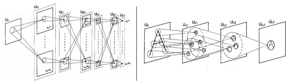
Although the neocognitron achieved some success in pattern recognition tasks and introduced convolutional filters to neural networks, it was limited by its lack of a training algorithm to learn the filters. This meant that the pattern detectors were manually engineered for the specific task, using a variety of heuristics and techniques from computer vision. At the time, backpropagation had not yet been applied to train neural nets, and thus there was no easy way to optimize neocognitrons or reuse them on different vision tasks.
LeNet (1998)
In the late 1980s, Geoffrey Hinton et al first succeeded in applying backpropagation to the training of neural networks. During the 1990s, a team at AT&T Labs led by Hinton’s former post-doc student Yann LeCun trained a convolutional network, nicknamed “LeNet”, to classify images of handwritten digits to an accuracy of 99.3%. Their system was used for a time to automatically read the numbers in 10-20% of checks printed in the US. LeNet had 7 layers, including two convolutional layers, with the architecture summarized in the below figure.
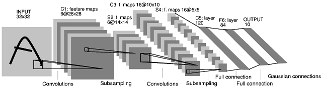
Their system was the first convolutional network to be applied on an industrial-scale application. Despite this triumph, many computer scientists believed that neural networks would be incapable of scaling up to recognition tasks involving more classes, higher resolution, or more complex content. For this reason, most applied computer vision tasks would continue to be carried out by other algorithms for more than another decade.
AlexNet (2012)
Convolutional networks began to take over computer vision – and by extension, machine learning more generally – in the early 2010s. In 2009, researchers at the computer science department at Princeton University, led by Fei-Fei Li, compiled the ImageNet database, a large-scale dataset containing over 14 million labeled images which were manually annotated into 1000 classes using Mechanical Turk. ImageNet was by far the largest such dataset ever released and quickly became a staple of the research community. A year later, the ImageNet Large Scale Visual Recognition Challenge (ILSVRC) was launched as an annual competition for computer vision researchers working with ImageNet. The ILSVRC welcomed researchers to compete on a number of important benchmarks, including classification, localization, detection, and others – tasks which will be described in more detail later in this chapter.

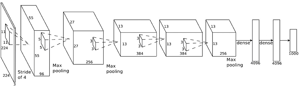
For the first two years of the competition, the winning entries all used what were then standard approaches to computer vision, and did not involve the use of convolutional networks. The top-winning entries in the classification tasks had a top-5 error (did not guess the correct class in top-5 predictions) between 25 and 28%. In 2012, a team from the University of Toronto led by Geoffrey Hinton, Ilya Sutskever, and Alex Krizhevsky submitted a deep convolutional neural network nicknamed “AlexNet” which won the competition by a dramatic margin of over 40%. AlexNet broke the previous record for top-5 classification error from 26% down to 15%.
Since the following year, nearly all entries to ILSVRC have been deep convolutional networks, and classification error has steadily tumbled down to nearly 2% in 2017, the last year of ILSVRC. Convnets now even outperform humans in ImageNet classification! These monumental results have largely fueled the excitement about deep learning that would follow, and many consider them to have revolutionized computer vision as a field outright. Furthermore, many important research breakthroughs that are now common in network architectures – such as residual layers – were introduced as entries to ILSVRC.
How convolutional layers work
Despite having their own proper name, convnets are not categorically different from the neural networks we have seen so far. In fact, they inherit all of the functionality of those earlier nets, and improve them mainly by introducing a new type of layer, called a convolutional layer, along with a number of other innovations emulating and refining the ideas introduced by neocognitron. Thus any neural network which contains at least one convolutional layer can be called a convolutional network.
Filters and activation maps
Prior to this chapter, we’ve just looked at fully-connected layers, in which each neuron is connected to every neuron in the previous layer. Convolutional layers break this assumption. They are actually mathematically very similar to fully-connected layers, differing only in the architecture. Let’s first recall that in a fully-connected layer, we compute the value of a neuron $z$ as a weighted sum of all the previous layer’s neurons, $z=b+\sum{w x}$.
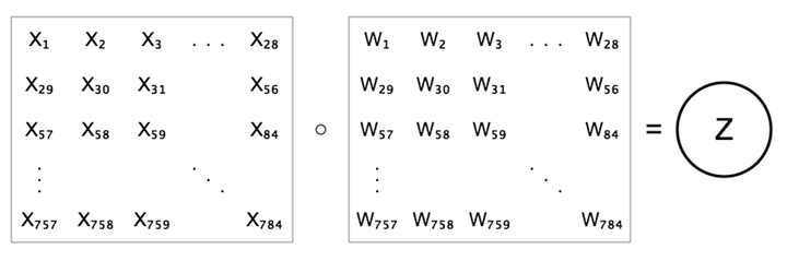
We can interpret the set of weights as a feature detector which is trying to detect the presence of a particular feature. We can visualize these feature detectors, as we did previously for MNIST and CIFAR. In a 1-layer fully-connected layer, the “features” are simply the the image classes themselves, and thus the weights appear as templates for the entire classes.
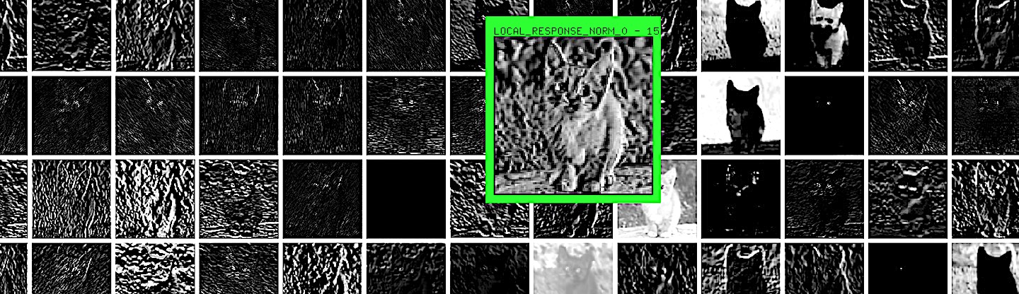
In convolutional layers, we instead have a collection of smaller feature detectors called convolutional filters which we individually slide along the entire image and perform the same weighted sum operation as before, on each subregion of the image. Essentially, for each of these small filters, we generate a map of responses–called an activation map–which indicate the presence of that feature across the image.
The process of convolving the image with a single filter is given by the following interactive demo.
In the above demo, we are showing a single convolutional layer on an MNIST digit. In this particular network at this layer, we have exactly 8 filters, and below we show each of the corresponding 8 activation maps.
Each of the pixels of these activation maps can be thought of as a single neuron in the next layer of the network. Thus in our example, since we have 8 filters generating $25 * 25$ sized maps, we have $8 * 25 * 25 = 5000$ neurons in the next layer. Each neuron signifies the amount of a feature present at a particular xy-point. It’s worth emphasizing the differences in our visualization above to what we have seen before; in prior chapters, we always viewed the neurons (activations) of ordinary neural nets as one long column, whereas now we are viewing them as a set of activation maps. Although we could also unroll these if we wish, it helps to continue to visualize them this way because it gives us some visual understanding of what’s going on. We will refine this point in a later section.
Convolutional layers have a few properties, or hyperparameters, which must be set in advance. They include the size of the filters ($5x5$ in the above example), the stride and spatial arrangement, and padding. A full explanation of these is beyond the scope of the chapter, but a good overview of these can be found here.
Pooling layers
Before we explain the significance of the convolutional layers, let’s also quickly introduce pooling layers, another (much simpler) kind of layer, which are very commonly found in convnets, often directly after convolutional layers. These were originally called “subsampling” layers by LeCun et al, but are now generally referred to as pooling.
The pooling operation is used to downsample the activation maps, usually by a factor of 2 in both dimensions. The most common way of doing this is max pooling which merges the pixels in adjacent 2x2 cells by taking the maximum value among them. The figure below shows an example of this.
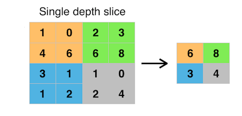
The advantage of pooling is that it gives us a way to compactify the amount of data without losing too much information, and create some invariance to translational shift in the original image. The operation is also very cheap since there are no weights or parameters to learn.
Recently, pooling layers have begun to gradually fall out of favor. Some architectures have incorporated the downsampling operation into the convolutional layers themselves by using a stride of 2 instead of 1, making the convolutional filters skip over pixels, and result in activation maps half the size. These “all-convolutional nets” have some important advantages and are becoming increasingly common, but have not yet totally eliminated pooling in practice.
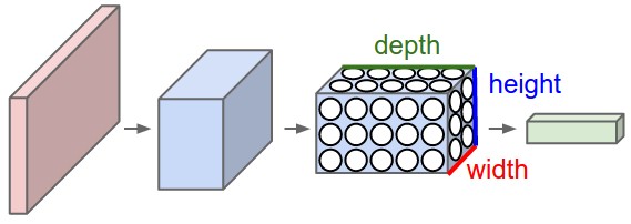
Volumes
Let’s zoom out from what we just looked at and see the bigger picture. From this point onward, it helps to interpret the data flowing through a convnet as a “volume,” i.e. a 3-dimensional data structure. In previous chapters, our visualizations of neural networks always “unrolled” the pixels into a long column of neurons. But to visualize convnets properly, it makes more sense to continue to arrange the neurons in accordance with their actual layout in the image, as we saw in the last demo with the eight activation maps.
In this sense, we can think of the original image as a volume of data. Let’s consider the previous example. Our original image is 28 x 28 pixels and is grayscale (1 channel). Thus it is a volume whose dimensions are 28x28x1. In the first convolutional layer, we convolved it with 8 filters whose dimensions are 5x5x1. This gave us 8 activation maps of size 24x24. Thus the output from the convolutional layer is size 24x24x8. After max-pooling it, it’s 12x12x8.
What happens if the original image is color? In this case, our analogy scales very simply. Our convolutional filters would then also be color, and therefore have 3 channels. The convolution operation would work exactly as it did before, but simply have three times as many multiplications to make; the multiplications continue to line up by x and y as before, but also now by channel. So suppose we were using CIFAR-10 color images, whose size is 32x32x3, and we put it through a convolutional layer consisting of 20 filters of size 7x7x3. Then the output would be a volume of 26x26x20. The size in the x and y dimensions is 26 because there are 26x26 possible positions to slide a 7x7 filter into inside of a 32x32 image, and its depth is 20 because there are 20 filters.
We can think of the stacked activation maps as a sort-of “image.” It’s no longer really an image of course because there are 20 channels instead of just 3, as there are in actual RGB images. But it’s worth seeing the equivalence of these representations; the input image is a volume of size 32x32x3, and the output from the first convolutional layer is a volume of size 26x26x20. Whereas the values in the 32x32x3 volume simply represent the intensity of red, green, and blue in every pixel of the image, the values in the 26x26x20 volume represent the intensity of 20 different feature detectors over a small region centered at each pixel. They are equivalent in that they are giving us information about the image at each pixel, but the difference is in the quality of the information. The 26x26x20 volume captures “high-level” information abstracted from the original RGB image.
Things get deep
Ok, here’s where things get tricky. In typical neural networks, we frequently have multiple convolutional (and pooling layers) arranged in a sequence. Suppose after our first convolution gives us the 26x26x20 volume, we attach another convolutional layer consisting of 30 new feature detectors, each of which are sized 5x5x20. Why is the depth 20? Because in order to fit, the filters have to have as many channels as the activation maps they are being convolved over. If there is no padding, each of the new filters will produce a new activation map of size 22x22. Since there are 30 of them, that means we’ll have a new volume of size 22x22x30.
How should these new convolutional filters and the resulting activation maps or volume be interpreted? These feature detectors are looking for patterns in the volume from the previous layer. Since the previous layer already gave us patterns, we can interpret these new filters as looking for patterns of those patterns. This can be hard to wrap your head around, but it follows straight from the logic of the idea of feature detectors. If the first feature detectors could detect only simple patterns like differently-oriented edges, the second feature detectors could combine those simple patterns into slightly more complex or “high-level” patterns, such as corners or grids.
And if we attach a third convolutional layer? Then the patterns found from that layer are yet higher-level patterns, perhaps things like lattices or very basic objects. Those basic objects can be combined in another convolutional layer to detect even more complex objects, and so on. This is the core idea behind deep learning: by continuously stacking these feature detectors on top of each other over many layers, we can learn a compositional hierarchy of features, from simple low-level patterns to complex high-level objects. The final layer is a classification, and it is likely to do much better learning from the high-level representation given to it by many layers, than it otherwise would do on the raw pixels or some hand-crafted statistical representation of them alone.
You may be wondering how are the filters determined? Recall that the filters are just collections of weights, just like all of the other weights we’ve discussed in previous chapters. They are parameters which are learned during the process of training. See the previous chapter on how neural nets are trained for a review of that process.
Improving CIFAR-10 accuracy
The following interactive figure shows a confusion matrix of a convolutional network trained to classify the CIFAR-10 dataset, achieving a very respectable 79% accuracy. Although the current state of the art for CIFAR-10 gets around 96%, our 79% result is quite impressive considering that it was trained on nothing more than a client-side, CPU-only, javascript library! Recall that an ordinary neural network with no convolutional layers only achieved 37% accuracy. So we can see the immense improvement that convolutional layers give us. By selecting the first menu, you can see confusion matrices for convnets and ordinary neural nets trained on both CIFAR-10 and MNIST.
Applications of convnets
Since the early 2010s, convnets have ascended to become the most widely used deep learning algorithms for a variety of applications. Once considered successful only for a handful of specific computer vision tasks, they are now also deployed for audio, text, and other types of data processing. They owe their versatility to the automation of feature extraction, something which was once the most time-consuming and costly process necessary for applying a learning algorithm to a new task. By incorporating feature extraction itself into the training process, it’s now possible to re-appropriate an existing convnet’s architecture, often with very few changes, into a totally different task or even different domain, and retrain or “fine-tune” it to the new task.
Although a full review of convnets many applications is beyond the scope of this chapter, this section will highlight a small number of them which are relevant to creative uses.
In computer vision
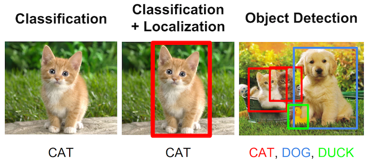
Besides for image classification, convnets can be trained to perform a number of tasks which give us more granular information about images. One task closely associated with classification is that of localization: assigning a bounding rectangle for the primary subject of the classification. This task is typically posed as a regression alongside the classification, where the network must accurately predict the coordinates of the box (x, y, width, and height).
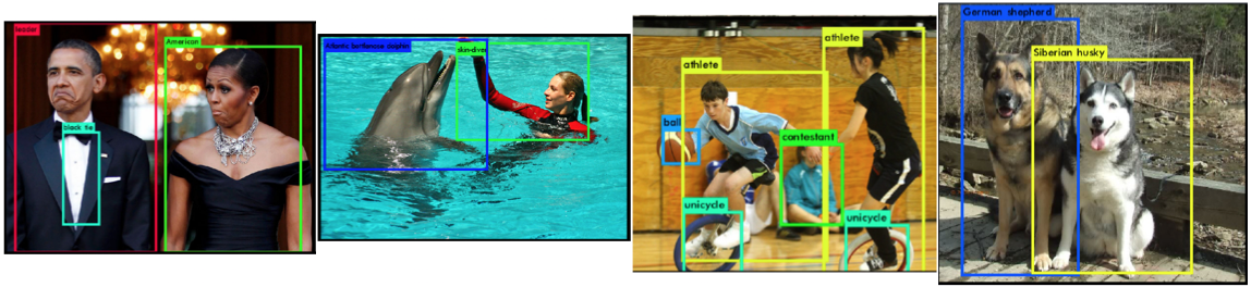
This task can be extended more ambitiously to the task of object detection. In object detection, rather than classifying and localizing a single subject in the image, we allow for the presence of multiple objects to be located and classified within the image. The below image summarizes these three associated tasks.
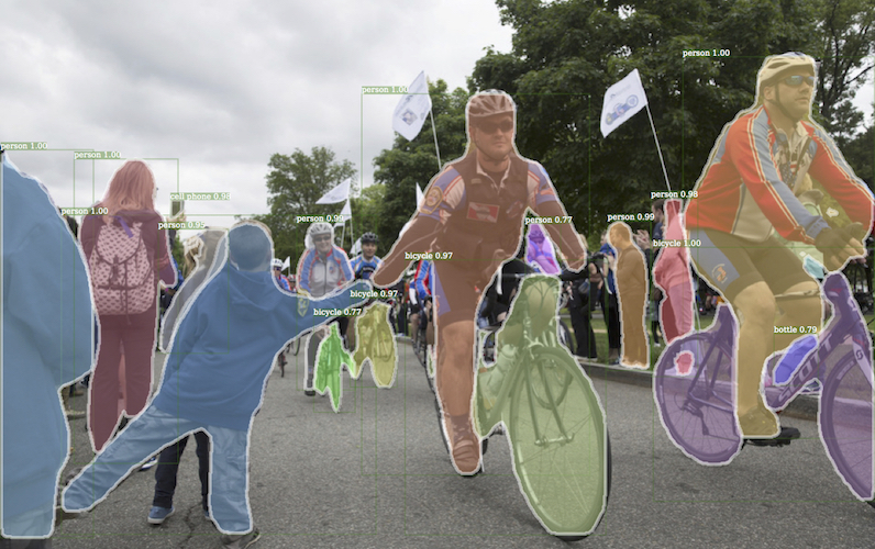
Closely related is the task of semantic segmentation, a task which involves segmenting an image into all its found objects. This is similar to object detection, but actually demarcates the full border of each found object, rather than just its bounding box.
Semantic segmentation and object detection have only become feasible relatively recently. One of the major limitations holding them back previously, besides for the increased complexity compared to single-class classification, was a lack of available data. Even the imagenet dataset, which was used to take classification to the next level, was unable to do anything about detection or segmentation because it had sparse information about the locations of objects. But more recent datasets like MS-COCO have added richer information for each image into their schema, enabling us to pursue localization, detection, and segmentation more seriously.
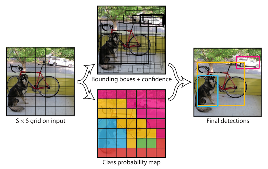
Early attempts at training convnets to do multiple object detection typically used a localization-like task to first identify potential bounding boxes, then simply applied classification to all of those boxes, keeping the ones in which it had the most confidence. This approach is very slow however because it requires at least one forward pass of the network for each of the dozens or even hundreds of candidates. In certain situations, such as with self-driving cars, this latency is obviously unacceptable. In 2016, Joseph Redmon developed YOLO to address these limitations. YOLO – which stands for “you only look once” – restricts the network to only “look” at the image a single time, i.e. it is permitted a single forward pass of the network to obtain all the information it needs, hence the name. It has in some circumstances achieved a 40-90 frames-per-second speed on multiple object detection, making it capable of being deployed in real-time scenarios demanding such responsiveness. The approach is to divide the image into a grid of equally-sized regions, and have each one predict a candidate object along with its classification and bounding box. At the end, those regions with the highest confidence are kept. The figure below summarizes this approach.
Still more tasks relevant to computer vision have been introduced or improved in the last few years, as well as systems specialized for retrieving text from images by combining convnets with recurrent neural networks (to be introduced in a later chapter). Another class of tasks involves annotating images with natural language by combining convnets with recurrent neural networks. This chapter will leave those to be discussed by future chapters, or within the included links for further reading.
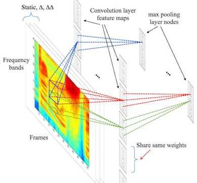
Audio applications
Perhaps one of the most surprising aspects about convnets is their versatility, and their success in the audio domain. Although most introductions to convnets (like this chapter) emphasize computer vision, convnets have been achieving state-of-the-art results in the audio domain for just as long. They are routinely used for speech recognition and other audio information retrieval work, supplanting older approaches over the last few years as well. Prior to the ascendancy of neural networks into the audio domain, speech-to-text was typically done using a hidden markov model along with handcrafted audio feature extraction done using conventional digital signal processing.
A more recent use case for convnets in audio is that of WaveNet, introduced by researchers at DeepMind in late-2016. WaveNets are capable of learning how to synthesize audio by training on large amounts of raw audio. WaveNets have been used by Magenta to create custom digital audio synthesizers and are now used to generate the voice of Google Assistant.
Generative applications of convnets, including those in the image domain and associated with computer vision, as well as those that also make use of recurrent neural networks, are left to future chapters.