Style transfer is the technique of recomposing one image in the style of another. Two inputs, a content image and a style image are analyzed by a convolutional neural network which is then used to create an output image whose “content” mirrors the content image and whose style resembles that of the style image. It was first demonstrated in the paper “A neural algorithm of artistic style” published by Gatys, Ecker, and Bethge at the University of Tübingen in August 2015, and has since continued to be of great interest to artists and scientists alike.

[Figure:: Tubingen photo]

In a more general context, style transfer can be taken to mean the same technique in any medium. One could imagine a program resynthesizing The Star Spangled Banner as heavy metal or bossa nova, or rewriting Harry Potter in the frantic tone of Edgar Allen Poe. Although so far it has only been demonstrated convincingly with images, there is much effort underway at developing it in the video, audio, and text domains. The capability is prized for its far-reaching applications, as well as the insights it could potentially provide into our perception of style.

Stylenet theory

Producing the output image

The objective of the style transfer algorithm is to find an output image, \(\vec x\), which minimizes a loss function that is the sum of two separate terms, a “content loss” and a “style loss.” We will define them in more detail shortly, but for now it suffices to say that the content loss denotes the content dissimilarity between the content image \(\vec p\) and the output image \(\vec x\), while the style loss is the style dissimilarity between the style image \(\vec a\) and the output image \(\vec x\). The total loss is given by:

\[\begin{eqnarray} L_{total}(\vec p, \vec a, \vec x) = \alpha L_{content}(\vec p,\vec x) + \beta L_{style}(\vec a,\vec x) \end{eqnarray}\]

Because the content loss and style loss are both functions of our output image’s pixels, it follows that they are in mutual conflict; no output image is likely to optimize both terms simultaneously. So \(\alpha\) and \(\beta\) are parameters that are used to control the relative importance of each term to us. By setting \(\alpha\) higher than \(\beta\), the loss function favors minimizing content loss over style loss, while setting \(\beta\) prioritizes style.

Like with Deepdream, the output pixels \(\vec x\) are determined by an iterative procedure in which at each step, we slightly adjust the output image’s pixels so as to decrease the loss. We do this repeatedly until the loss stops lowering or your mind is blown. We typically initialize the output image randomly with white noise or we copy the content image, as in the case of Deepdream.

The iterative procedure used is the standard gradient descent in which we calculate the gradient of the loss with respect to the pixels, and then adjust them to decrease the loss. This is in fact the same procedure which is used to train neural networks! The only difference is that instead of adjusting weights, we are adjusting pixels. The prior chapter, “How neural networks are trained”, explains gradient descent more thoroughly.

The following two examples shows the generation of an output image from transferring the style of __ onto __, The top one sets \(\alpha\) higher than \(\beta\), thus favoring content similarity over style similarity, whereas the bottom does vice-versa. We can see that bottom result appears to have less of the original content preserved, but does a better job of capturing the style.

figure which explains both the iterative process and alpha/beta [Figure: animation of iterations of producing output image with high alpha ] [Figure: animation of iterations of producing output image with high beta ]

Content loss

Both the content loss and style loss are determined from the activations of a trained convolutional neural network. Recall that a convnet’s activations are arranged as a series of feature maps which reflect the presence of different features within the image, where features have a progressively higher-level or more abstract composition at each layer of the convnet. To fully appreciate how the loss terms are derived, it will help to review the prior chapters on convolutional neural networks, and especially how to interpret the activations.

[ visuals of convnet ]

The content loss is calculated in the following way. Both the output image and content image are run through a convnet, giving us a set of feature maps for both. The loss at a single layer is the euclidean (L2) distance between the activations of the content image and the activations of the output image.

\[\begin{eqnarray} L_{content}(\vec p, \vec x, l) = \frac {1}{2} \sum_{i,j} (F_{ij}^l - P_{ij}^l)^2 \end{eqnarray}\]

_ The loss function for the content similarity is simply the distance between the synthetic image’s activations and the style image’s activations. In principle, this can be any or all of the activations, though in practice, most implementations choose one of the intermediate layers to compute this over.
_

Style loss

Like the content loss, style loss is also a function of the convnet’s activations, but is slightly more complex. We pass the style image and output image through a convnet and observe their activations. But instead of comparing the raw activations directly, we add another step. For both images, we take the Gram matrix of the activations at each layer in the network. For a single image, the Gram matrix of its activations at a layer \(l\) is given by:

\[\begin{eqnarray} G_{ij}^l = {F_i^l} \cdot {F_j^l} \end{eqnarray}\]

where \(F_i^l\) and \(F_j^l\) are the activations for the i-th and j-th feature maps at layer \(l\), and \({F_i^l} \cdot {F_j^l}\) is the dot product between them, correlation. In other words, the resulting matrix, \(G^l\) contains the correlations between every pair of feature maps at layer \(l\) for that image.

For reasons that can only be regarded as magic, this turns out to be a very good representation of our perception of style within images. It captures the tendency of features to co-occur in different parts of the image.

After calculating those, we can define the style loss at a single layer \(l\) as the euclidean (L2) distance between the Gram matrices of the style and output images.

\[\begin{eqnarray} E_l = \frac {1}{4N_l^2 M_l^2} \sum_{i,j} (G_{ij}^l - A_{ij}^l)^2 \end{eqnarray}\]

The main part of the above formula is the summation term which gives us the total element-wise distance between the Gram matrices of the style and output images. The constant \(\frac {1}{4N_l^2 M_l^2}\) is a normalization term.

Finally, we can compute the total style loss as a weighted sum of the style loss at each layer.

\[\begin{eqnarray} L_{style}(\vec a,\vec x) = \sum_{l} {w_l}{E_l} \end{eqnarray}\]

The weights for each layer’s loss \({w_l}\) are another hyperparameter for us to freely choose. Since the features at each layer of the network are progressively higher-level and more abstract, the style loss at each layer is also as such….

Implementations and artworks

Several independent implementations appeared after the publication of the paper.

Following the release of these implementations, many people contributed numerous … including the author.

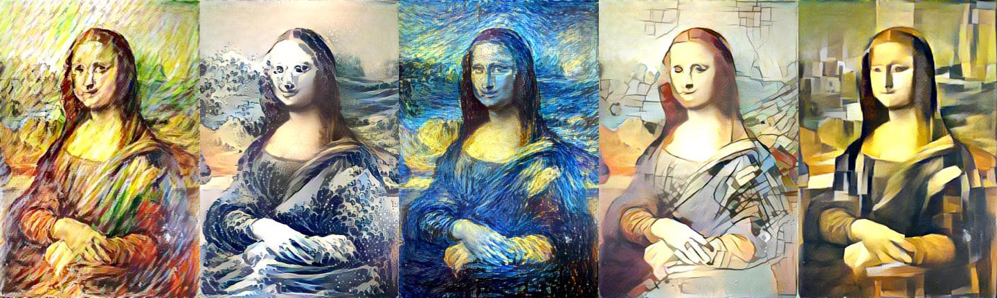
Gallery:

Video

What if there’s no content image?

Deep texture

Style interpolation

We can make the algorithm produce images with multiple styles evident by averaging the Gram matrices of several style inputs. The averages can be weighted, giving more influence to one or more of the styles.

[Picasso x Picasso]

Tutorial

implementations style loss vs content loss what do the parameters do

Style transfer in other domains

neural doodle neural-doodle2.png

style is a nebulous term

works by others

• deep forger
• style studies
• starry night in nyc
• deepart.io
• twitter #stylenet

john mccarthy 1955 coined AI turing 50 - computing machine and intelligence

graph of imagenet top accuracy, ILSVRC, Russakovsky et al 2015

convnet from the top – big tiles to small tiles single differentiable function

captioning: conditioning an RNN via convnet activations from training in which we associate states of the convnet and rnn learns more meaning iteratively

SHRDLU

• put the box on a pyraimd

computer reads recipes and robot is trained to perform it

• same crossmodal properties

olga russakovsky richard socher

audio style transfer igor ulyanov

https://arxiv.org/abs/1703.07511 https://arxiv.org/pdf/1307.3581.pdf

https://harishnarayanan.org/writing/artistic-style-transfer/