Imagine you are a mountain climber on top of a mountain, and night has fallen. You need to get to your base camp at the bottom of the mountain, but in the darkness with only your dinky flashlight, you can’t see more than a few feet of the ground in front of you. So how do you get down? One strategy is to look in every direction to see which way the ground steeps downward the most, and then step forward in that direction. Repeat this process many times, and you will gradually go farther and farther downhill. You may sometimes get stuck in a small trough or valley, in which case you can follow your momentum for a bit longer to get out of it. Caveats aside, this strategy will eventually get you to the bottom of the mountain.
This scenario may seem disconnected from neural networks, but it turns out to be a good analogy for the way they are trained. So good in fact, that the primary technique for doing so, gradient descent, sounds much like what we just described. Recall that training refers to determining the best set of weights for maximizing a neural network’s accuracy. In the previous chapters, we glossed over this process, preferring to keep it inside of a black box, and look at what already trained networks could do. The bulk of this chapter however is devoted to illustrating the details of how gradient descent works, and we shall see that it resembles the climber analogy we just described.
Neural networks can be used without knowing precisely how training works, just as one can operate a flashlight without knowing how the electronics inside it work. Most modern machine learning libraries have greatly automated the training process. Owing to those things and this topic being more mathematically rigorous, you may be tempted to set it aside and rush to applications of neural networks. But the intrepid reader knows this to be a mistake, because understanding the process gives valuable insights into how neural nets can be applied and reconfigured. Moreover, the ability to train large neural networks eluded us for many years and has only recently become feasible, making it one of the great success stories in the history of AI, as well as one of the most active and interesting research areas.
The aim of this chapter is to give an intuitive, if not rigorous understanding of how neural networks are solved. Visuals are preferred over equations wherever possible, and external links for further reading and refinement will be offered along the way. We’ll get to gradient descent, backpropagation, and all the techniques involved in a few sections, but first, let’s understand why training is hard to begin with.
Why training is hard
A needle in a hyper-dimensional haystack
The weights of a neural network with hidden layers are highly interdependent. To see why, consider the highlighted connection in the first layer of the three layer network below. If we tweak the weight on that connection slightly, it will impact not only the neuron it propagates to directly, but also all of the neurons in the next two layers as well, and thus affect all the outputs.
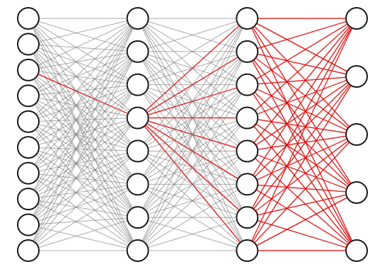
For this reason, we know we can’t obtain the best set of weights by optimizing one at a time; we will have to search the entire space of possible weight combinations simultaneously. How do we do this?
Let’s start with the simplest, most naive approach to picking them: random guesses. We set all the weights in our network to random values, and evaluate its accuracy on our dataset. Repeat this many times, keeping track of the results, and then keep the set of weights that gave us the most accurate results. At first this may seem like a reasonable approach. After all, computers are fast; maybe we can get a decent solution by brute force. For a network with just a few dozen neurons, this would work fine. We can try millions of guesses quickly and should get a decent candidate from them. But in most real-world applications we have a lot more weights than that. Consider our handwriting example from the previous chapter. There are around 12,000 weights in it. The best combination of weights among that many is now a needle in a haystack, except that haystack has 12,000 dimensions!
You might be thinking that 12,000-dimensional haystack is “only 4,000 times bigger” than the more familiar 3-dimensional haystack, so it ought to take only 4,000 times as much time to stumble upon the best weights. But in reality the proportion is incomprehensibly greater than that, and we’ll see why in the next section.
n-dimensional space is a lonely place
If our strategy is brute force random search, we may ask how many guesses will we have to take before we obtain a reasonably good set of weights. Intuitively, we should expect that we need to take enough guesses to sample the whole space of possible guesses densely; with no prior knowledge, the correct weights could be hiding anywhere, so it makes sense to try to sample the space as much as possible.
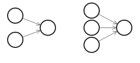
To illustrate this, let’s consider two very small 1-layer neural networks, the first one with 2 neurons, and the second one with 3 neurons. For the sake of simplicity, we will ignore the bias for the moment.
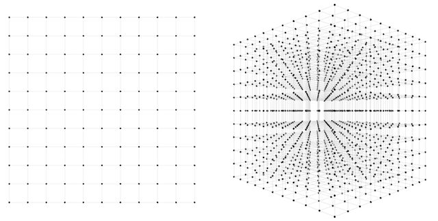
In the first network, there are 2 weights to find. How many guesses should we take to be confident that one of them will lead to a good fit? One way to approach this question is to imagine the 2-dimensional space of possible weight combinations and exhaustively search through every combination to some level of granularity. Perhaps we can take each axis and divide it into 10 segments. Then our guesses would be every combination of the two; 100 in all. Not so bad; sampling at such density covers most of the space pretty well. If we divide the axes into 100 segments instead of 10, then we have to make 100*100=10,000 guesses, and cover the space very densely. 10,000 guesses is still pretty small; any computer will get through that in less than a second.
How about the second network? Here we have three weights instead of two, and therefore a 3-dimensional space to search through. If we want to sample this space to the same level of granularity that we sampled our 2d network, we again divide each axis into 10 segments. Now we have 10 * 10 * 10 = 1,000 guesses to make. Both the 2d and 3d scenarios are depicted in the below figure.
1,000 guesses is a piece of cake, we might say. At a granularity of 100 segments, we would have \(100 * 100 * 100 = 1000000\) guesses. 1,000,000 guesses is still no problem, but now perhaps we are getting nervous. What happens when we scale up this approach to more realistic sized networks? We can see that the number of possible guesses blows up exponentially with respect to the number of weights we have. In general, if we want to sample to a granularity of 10 segments per axis, then we need \(10^N\) samples for an \(N\)-dimensional dataset.
So what happens when we try to use this approach to train our network for classifying MNIST digits from the first chapter? Recall that network has 784 input neurons, 15 neurons in 1 hidden layer, and 10 neurons in the output layer. Thus, there are \(784*15 + 15*10 = 11910\) weights. Add 25 biases to the mix, and we have to simultaneously guess through 11,935 dimensions of parameters. That means we’d have to take \(10^{11935}\) guesses… That’s a 1 with almost 12,000 zeros after it! That is an unimaginably large number; to put it in perspective, there are only \(10^{80}\) atoms in the entire universe. No supercomputer can ever hope to perform that many calculations. In fact, if we took all of the computers existing in the world today, and left them running until the Earth crashed into the sun, we still wouldn’t even come close! And just consider that modern deep neural networks frequently have tens or hundreds of millions of weights.
This principle is closely related to what we call in machine learning “the curse of dimensionality.” Each dimension we add into a search space exponentially blows up the number of samples we require to get good generalization for any model learned from it. The curse of dimensionality is more often applied to datasets; simply put, the more columns or variables a dataset is represented with, the exponentially more samples in that dataset we need to understand it. In our case, we are thinking about the weights rather than the inputs, but the principle remains the same; high-dimensional space is enormous!
Obviously there needs to be some more elegant solution to this problem than random guesses. In order to build up our understanding of an efficient computational method for solving such a problem, let’s again forget about neural networks for a minute, and start instead with a simpler problem and scale up gradually until we’ve reinvented gradient descent.
Linear regression
Linear regression refers to the task of determining a “line of best fit” through a set of data points and is a simple predecessor to the more complex nonlinear methods we use to solve neural networks. This section will show you an example of linear regression. Suppose we are given a set of 7 points, those in the chart to the bottom left. To the right of the chart is a scatterplot of our points.
| 2.4 | 1.7 |
| 2.8 | 1.85 |
| 3.2 | 1.79 |
| 3.6 | 1.95 |
| 4.0 | 2.1 |
| 4.2 | 2.0 |
| 5.0 | 2.7 |
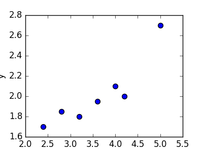
The goal of linear regression is to find a line which best fits these points. Recall that the general equation for a line is \(f(x) = m \cdot x + b\), where \(m\) is the slope of the line, and \(b\) is its y-intercept. Thus, solving a linear regression is determining the best values for \(m\) and \(b\), such that \(f(x)\) gets as close to \(y\) as possible. Let’s try out a few random candidates.
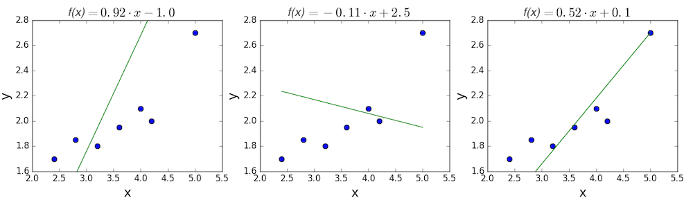
Pretty clearly, the first two lines don’t fit our data very well. The third one appears to fit a little better than the other two. But how can we decide this? Formally, we need some way of expressing how good the fit is, and we can do that by defining a loss function.
Loss function
The loss function – sometimes called a cost function – is a measure of the amount of error our linear regression makes on a dataset. Although many loss functions exist, all of them essentially penalize us on the distance between the predicted y-value from a given \(x\) and its actual value in our dataset. For example, taking the line from the middle example above, \(f(x) = -0.11 \cdot x + 2.5\), we highlight the error margins between the actual and predicted values with red dashed lines.
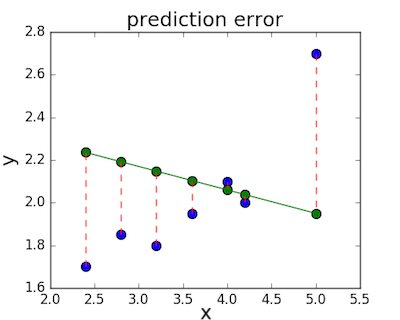
One very common loss function is called mean squared error (MSE). To calculate MSE, we simply take all the error bars, square their lengths, and take their average.
\[MSE = \frac{1}{n} \sum_i{(y_i - f(x_i))^2}\] \[MSE = \frac{1}{n} \sum_i{(y_i - (mx_i + b))^2}\]We can go ahead and calculate the MSE for each of the three functions we proposed above. If we do so, we see that the first function achieves a MSE of 0.17, the second one is 0.08, and the third gets down to 0.02. Not surprisingly, the third function has the lowest MSE, confirming our guess that it was the line of best fit.
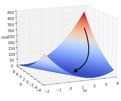
We can get some intuition if we calculate the MSE for all \(m\) and \(b\) within some neighborhood and compare them. Consider the figure below, which uses two different visualizations of the mean squared error in the range where the slope \(m\) is between -2 and 4, and the intercept \(b\) is between -6 and 8.
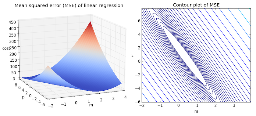
Right: the same figure, but visualized as a 2-d contour plot where the contour lines are logarithmically distributed height cross-sections.
Looking at the two graphs above, we can see that our MSE is shaped like an elongated bowl, which appears to flatten out in an oval very roughly centered in the neighborhood around \((m,p) \approx (0.5, 1.0)\). In fact, if we plot the MSE of a linear regression for any dataset, we will get a similar shape. Since we are trying to minimize the MSE, we can see that our goal is to figure out where the lowest point in the bowl lies.
Adding more dimensions
The above example is quite minimal, having just one independent variable, \(x\), and thus two parameters, \(m\) and \(b\). What happens when there are more variables? In general, if there are \(n\) variables, a linear function of them can be written out as:
\[f(x) = b + w_1 \cdot x_1 + w_2 \cdot x_2 + ... + w_n \cdot x_n\]Or in matrix notation, we can summarize it as:
\[f(x) = b + W^\top X \;\;\;\;\;\;\;\;where\;\;\;\;\;\;\;\; W = \begin{bmatrix} w_1\\w_2\\\vdots\\w_n\\\end{bmatrix} \;\;\;\;and\;\;\;\; X = \begin{bmatrix} x_1\\x_2\\\vdots\\x_n\\\end{bmatrix}\]One trick we can use to simplify this is to think of our bias $b$ as being simply another weight, which is always being multiplied by a “dummy” input value of 1. In other words, we let:
\[f(x) = W^\top X \;\;\;\;\;\;\;\;where\;\;\;\;\;\;\;\; W = \begin{bmatrix} b\\w_1\\w_2\\\vdots\\w_n\\\end{bmatrix} \;\;\;\;and\;\;\;\; X = \begin{bmatrix} 1\\x_1\\x_2\\\vdots\\x_n\\\end{bmatrix}\]This equivalent formulation is convenient both notationally, since now our function is more simply expressed as $f(x) = W^\top X$, and conceptually, since we can now think of the bias as just another weight, and therefore just one more parameter that needs to be optimized.
Adding many more dimensions may seem at first to complicate our problem horribly, but it turns out that the formulation of the problem remains exactly the same in 2, 3, or any number of dimensions. Although it is impossible for us to draw it now, there exists a loss function which appears like a bowl in some number of dimensions – a hyper-bowl! And as before, our goal is to find the lowest part of that bowl, objectively the smallest value that the loss function can have with respect to some parameter selection and dataset.
So how do we actually calculate where that point at the bottom is exactly? There are numerous ways to do so, with the most common approach being the ordinary least squares method, which solves it analytically. When there are only one or two parameters to solve, this can be done by hand, and is commonly taught in an introductory course on statistics or linear algebra.
The curse of nonlinearity
Alas, ordinary least squares cannot be used to optimize neural networks however, and so solving the above linear regression will be left as an exercise left to the reader. The reason we cannot use linear regression is that neural networks are nonlinear; Recall the essential difference between the linear equations we posed and a neural network is the presence of the activation function (e.g. sigmoid, tanh, ReLU, or others). Thus, whereas the linear equation above is simply \(y = b + W^\top X\), a 1-layer neural network with a sigmoid activation function would be \(f(x) = \sigma (b + W^\top X)\).
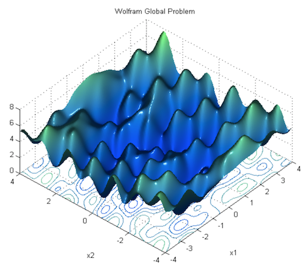
This nonlinearity means that the parameters do not act independently of each other in influencing the shape of the loss function. Rather than having a bowl shape, the loss function of a neural network is more complicated. It is bumpy and full of hills and troughs. The property of being “bowl-shaped” is called convexity, and it is a highly prized convenience in multi-parameter optimization. A convex loss function ensures we have a global minimum (the bottom of the bowl), and that all roads downhill lead to it.
But by introducing the nonlinearity, we lose this convenience for the sake of giving our neural networks much more “flexibility” in modeling arbitrary functions. The price we pay is that there is no easy way to find the minimum in one step analytically anymore (i.e. by deriving neat equations for them). In this case, we are forced to use a multi-step numerical method to arrive at the solution instead. Although several alternative approaches exist, gradient descent remains the most popular and effective. The next section will go over how it works.
Gradient Descent
The general problem we’ve been dealing with – that of finding parameters to satisfy some objective function – is not specific to machine learning. Indeed it is a very general problem found in mathematical optimization, known to us for a long time, and encountered in far more scenarios than just neural networks. Today, many problems in multivariable function optimization – including training neural networks – generally rely on a very effective algorithm called gradient descent to find a good solution much faster than taking random guesses, and more powerful than linear regression.
The gradient descent method
Intuitively, the way gradient descent works is similar to the mountain climber analogy we gave in the beginning of the chapter. First, we start with a random guess at the parameters, and start there. We then figure out which direction the loss function steeps downward the most (with respect to changing the parameters), and step slightly in that direction. To put it another way, we determine the amounts to tweak all of the parameters such that the loss function goes down by the largest amount. We repeat this process over and over until we are satisfied we have found the lowest point.
To figure out which direction the loss steeps downward the most, it is necessary to calculate the gradient of the loss function with respect to all of the parameters. A gradient is a multidimensional generalization of a derivative; it is a vector containing each of the partial derivatives of the function with respect to each variable. In other words, it is a vector which contains the slope of the loss function along every axis.
Although we’ve already said that the most convenient way to solve linear regression is via ordinary least squares or some other single-step method, let’s quickly turn our attention back to linear regression to see a simple example of using gradient descent to solve a linear regression.
Recall the mean squared error loss we introduced in the previous section, which we will denote as $J$.
\[J = \frac{1}{n} \sum_i{(y_i - (mx_i + b))^2}\]There are two parameters we are trying to optimize: $m$ and $b$. Let’s calculate the partial derivative of $J$ with respect to each of them.
\[\frac{\partial J}{\partial m} = \frac{2}{n} \sum_i{x_i \cdot (y_i - (mx_i + b))}\] \[\frac{\partial J}{\partial b} = \frac{2}{n} \sum_i{(y_i - (mx_i + b))}\]How far in that direction should we step? This turns out to be an important consideration, and in ordinary gradient descent, this is left as a hyperparameter to decide manually. This hyperparameter – known as the learning rate – is generally the most important and sensitive hyperparameter to set and is often denoted as \(\alpha\). If \(\alpha\) is set too low, it may take an unacceptably long time to get to the bottom. If \(\alpha\) is too high, we may overshoot the correct path or even climb upwards.
Denoting the assignment operation as $:=$, we can write the update steps for the two parameters as follows.
\[m := m - \alpha \cdot \frac{\partial J}{\partial m}\] \[b := b - \alpha \cdot \frac{\partial J}{\partial b}\]If we take this approach to solving the simple linear regression we posed above, we will get something that looks like this:
And if there are more dimensions? If we denote all of our parameters as $w_i$, thus giving us the form $f(x) = b + W^\top X $, then we can extrapolate the above example to the multidimensional case. This can be written down more succinctly using gradient notation. Recall that the gradient of $J$, which we will denote as $\nabla J$, is the vector containing each of the partial derivatives. Thus we can represent the above update step as:
\[\nabla J(W) = \Biggl(\frac{\partial J}{\partial w_1}, \frac{\partial J}{\partial w_2}, \cdots, \frac{\partial J}{\partial w_N} \Biggr)\] \[W := W - \alpha \nabla J(W)\]The above formula is the canonical formula for ordinary gradient descent. It is guaranteed to get you the best set of parameters for a linear regression, or indeed for any linear optimization problem. If you understand the significance of this formula, you understand “in a nutshell” how neural networks are trained. In practice however, certain things complicate this process in neural networks and the next section will get into how we deal with them.
Applying gradient descent to neural nets
The problem of convexity
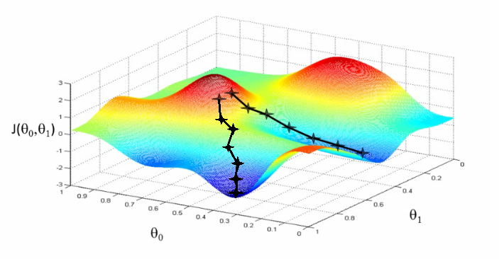
In the previous section, we showed how to run gradient descent for a simple linear regression problem, and declared that doing so is guaranteed to find the correct parameters. This is true for optimizing a linear model as we did, but it’s not true for neural networks, due to the nonlinearity introduced by their activation functions. Consequently, the loss function of a neural net is not “bowl-shaped”, and it is not convex. Instead, its loss function is much more complex, with many hills and valleys and curves and other irregularities. This means there are many “local minima” i.e. parameterizations where the loss is the lowest in its own immediate neighborhood, but not necessarily the absolute minimum (or “global minimum”). This means that if we run gradient descent, we might accidentally get stuck in a local minimum.
For theoretical reasons beyond the scope of this book, it turns out that this is not a major problem in deep learning, because when there are enough hidden units alongside some other criteria, most local minima are “good enough,” being reasonably close to the absolute minimum. According to Dauphin et al, a bigger challenge than local minima are saddle points, along which the gradient becomes very close to 0. For an explanation of why this is true, see this lecture by Yoshua Bengio (beginning at section 28, 1:09:41).
Despite the fact that local minima are not a major problem, we’d still prefer to overcome them to the extent they are any problem at all. One way of doing this is to modify the way gradient descent works, which is what the next section is about.
Stochastic, batch, and mini-batch gradient descent
Besides for local minima, “vanilla” gradient descent has another major problem: it’s too slow. A neural net may have hundreds of millions of parameters; this means a single example from our dataset requires hundreds of millions of operations to evaluate. Subsequently, gradient descent evaluated over all of the points in our dataset – also known as “batch gradient descent” – is a very expensive and slow operation. Moreover, because every dataset has inherent redundancy, it can be shown that a large enough subset of points can approximate the full gradient anyway, making batch gradient descent unnecessarily expensive to estimate the gradient.
It turns out that we can combat both this problem and the problem of local minima using a modified version of gradient descent called stochastic gradient descent (SGD). With SGD, we shuffle our dataset, and then go through each sample individually, calculating the gradient with respect to that single point, and performing a weight update for each. This may seem like a bad idea at first because a single example may be an outlier and not necessarily give a good approximation of the actual gradient. But it turns out that if we do this for each sample of our dataset in some random order, the overall fluctuations of the gradient update path will average out and converge towards a good solution. Moreover, SGD helps us get out of local minima and saddle points by making the updates more “jerky” and erratic, which can be enough to get unstuck if we find ourselves in the bottom of a valley.
SGD is particularly useful in cases where the loss surface is especially irregular. But in general, the usual approach is to use what is called mini-batch gradient descent (MB-GD), in which the whole dataset is randomly subdivided into \(N\) equally-sized mini-batches of \(K\) samples each. \(K\) may be a small positive number, or it can be in the dozens or hundreds; it depends on the specific architecture and application. Note that if \(K=1\), then you have SGD, and if \(K\) is the size of the whole dataset, it is batch gradient descent. Note also that confusingly, sometimes people say “SGD” to refer to both MB-GD and one sample at a time.
With MB-GD, we get the best of both worlds; the gradient is smoother and more stable than SGD, and reasonably similar to the full gradient, but we have a massive speed-up from not having to evaluate every sample in the dataset for each update. MB-GD is also computed very efficiently owing to parallelizable matrix operations.
In practice, MB-GD and SGD work well at efficiently optimizing the loss function of a neural network. However, they have weaknesses as well.
- The aforementioned problem of saddle points; we can get stuck in a parameterization where the loss function plateaus, and the gradient gets very close to 0.
- The learning rate remains a hyperparameter which must be set manually, which can be difficult to do. A learning rate which is too low leads to slow convergence, and one which is too high may overshoot the correct path.
Momentum
Momentum refers to a family of gradient descent variants where the weight update has inertia. In other words, the weight update is no longer a function of just the gradient at the current time step, but is gradually adjusted from the rate of the previous update.
Recall that in standard gradient descent, we calculate the gradient \(\nabla J(W)\) and use the following parameter update formula with learning rate \(\alpha\).
\[W_{t} := W_{t} - \alpha \nabla J(W_{t})\]Note that we’ve appended the \(t\) subscript to denote the current time step, which was previously omitted. In contrast, the generic formula for gradient descent with momentum is the following:
\[z_{t} := \beta z_{t-1} + \nabla J(W_{t-1})\] \[W_{t} := W_{t-1} - \alpha z_{t}\]In the parameter update, we’ve replaced the gradient \(\nabla J(W_{t})\) with a more complex function \(z_{t}\) that takes into account the gradient in past time steps. The higher \(\beta\) is set, the more momentum our parameter update is. If we set \(\beta = 0\), then the formula reverts to ordinary gradient descent. \(\alpha\) controls the overall learning rate of the process, as before.
You can think of the update path as being like a ball rolling downhill. Even if it gets to a region where the gradient changes significantly, it will continue going in roughly the same direction under its own momentum, only changing gradually along the path of the gradient. Momentum helps us escape saddle points and local minima by rolling out from them via speed built up from previous updates. It also helps counteract against the common problem of zig-zagging found along locally irregular loss surfaces where the gradient steeps strongly along some directions and not others.
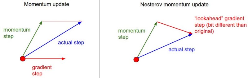
One alternative to the standard momentum formula is Nesterov accelerated gradient descent, given below:
\[z_{t} := \beta z_{t-1} + \nabla J(W_{t-1} - \beta z_{t-1} )\]The only change is, rather than evaluating the gradient where we currently are (\(W_{t-1}\)), we instead evaluate it at approximately where we will be at the next time step (\(W_{t-1} - \beta z_{t-1}\)), given the buildup of momentum carrying us in that direction. Calculating the gradient at that point instead of where we are currently lets us anticipate the loss surface ahead better and tune the momentum term accordingly. An illustration is given below:
Momentum methods work pretty well, but like MB-GD and SGD use a single formula for the entire gradient, despite any internal asymmetries among parameters. In contrast, methods which adapt to each element in the gradient have some advantages, which will be looked at in the next section. The following article at distill.pub looks at momentum in much more mathematical depth and nicely illustrates why it works.
Adaptive methods
Momentum comes in many flavors, and in general, finding fast, efficient, and accurate strategies for updating the parameters during gradient descent is a core objective of scientific research in the area, and a full discussion of them is out of the scope of this book. This section will instead quickly survey several of the more prominent variations in practical implementation, and refer to other materials online for a more comprehensive review.
One of the bigger annoyances in the training process is setting the learning rate \(\alpha\). Typically, an initial \(\alpha\) is set at the beginning, and is left to decay gradually over some number of time steps, letting it converge more precisely to a good solution. \(\alpha\) is the same for each individual parameter.
This is unsatisfactory because it assumes that the learning rate must follow a set schedule which is identical for each individual parameter, irrespective of the particular characteristics of the loss surface at a given time step. Additionally, it’s unclear how to set \(\alpha\) and its decay rate in the first place. Momentum and Nesterov momentum help to reduce this burden by giving the update rate some dependence on local observations rather than the “one-size-fits-all” approach of vanilla gradient descent. Still, the choice of \(\alpha\) and the inflexibility across parameters is seen as a problem.
A number of methods address this shortcoming by adapting the learning rate to each parameter individually, based on the assumption that there is a lot of variance of the loss across all the parameters. The simplest per-parameter update method is AdaGrad (standing for “Adaptive subGradient”). With AdaGrad, each parameter is updated individually according to its own gradient, but with a new coefficient which attempts to equalize the learning rate between parameters which tend towards large gradients and those that tend to small ones. AdaGrad is defined in the following formula (Note: for the sake of avoiding confusion, note the subscript \(i\) refers to index of the weight, rather than the time step as before ).
\[w_{i} := w_{i} - \frac{\alpha}{\sqrt{G_{i}+\epsilon}} \frac{\partial J}{\partial w_{i}}\]\(\sqrt{G_{i}+\epsilon}\) represents the sum of the squares of the gradient for that paramter for each step since training began (the \(\epsilon\) term is just some very small number, e.g. \(10^{-8}\), to avoid division-by-zero). By dividing \(\alpha\) for each parameter according to that quantity, we effectively slow down the learning rate for those parameters which have enjoyed large gradients up to that point, and conversely, speed up learning for parameters with minor or sparse gradients.
AdaGrad mostly eliminates the need to treat the initial learning rate \(\alpha\) as a hyperparameter, but it has its own challenges as well. The typical problem with AdaGrad is that learning may stop prematurely as \(G_{i}\) accumulates for each parameter over time and reduces the magnitude of the updates. A variant of AdaGrad, AdaDelta, addresses this by effectivly restricting the window of the gradient accumulation term to the most recent updates. Another adaptive method which is very similar to AdaDelta is RMSprop. RMSprop – proposed by Geoffrey Hinton during his Coursera class but otherwise unpublished – similarly shortsights the update by summing the squares of the previous updates, but does so in a simpler way by using a standard easing formula with a decay rate (which ends up being a hyperparameter). Thus, for both AdaDelta and RMSprop the update is not just adaptive with respect to parameters, but it’s adaptive with respect to time as well, instead of having the learning rate decay monotonically until stopping.
Adam and comparison of update methods
The last method worth mentioning in this chapter, and one of the most recent to be proposed, is Adam, whose name is derived from adaptive moment estimation. Adam gives us the best of both worlds between adaptive methods and momentum-based methods. Like AdaDelta and RMSprop, Adam adapts the learning rate for each parameter according to a sliding window of past gradients, but it has a momentum component to smooth the path over time steps.
Still more methods exist, and a full discussion of them is out of the scope of this chapter. A more complete discussion of them, including derivations and practical tips, can be found in this blog post by Sebastian Ruder.
This nice visualization, courtesy of Alec Radford, shows the characteristic behavior among the different gradient update methods discussed so far. Notice that momentum-based methods, Momentum and Nesterov accelerated gradient descent (NAG), tend to overshoot the optimal path by “rolling downhill” too fast, whereas standard SGD moves in the right path, but too slowly. Adaptive methods – AdaGrad, AdaDelta, and RMSProp (and we could add Adam to it as well) – tend to have the per-parameter flexibility to avoid both of those trappings.
So which optimization method works best? There’s no simple answer to this, and the answer largely depends on the characteristics of your data and other training constraints and considerations. Nevertheless, Adam has emerged as a promising method to at least start with. When data is sparse or unevenly distributed, the purely adaptive methods tend to work best. A full discussion of when to use each method is beyond the scope of this chapter, and is best found in the academic papers on optimizers, or in practical summaries such as this one by Yoshua Bengio.
For further reading on gradient descent optimization, see the following:
Hyperparameters and evaluation
Now that we understand the notion of optimizing the parameters of a network, we are ready to summarize the full procedure. The naive way to train our final model would be to run the gradient descent procedure over our full data. But we run into a problem if we do this: how do we evaluate the accuracy of our model? Since we’ve used up all our labeled data for training, the only way to evaluate it is to run the model on our training set again, and measure the difference between the output and the “ground truth” (the given labels). To understand why this is a bad practice, it is necessary to understand the phenomenon of overfitting.
Overfitting
Overfitting describes the situation in which your model is over-optimized to accurately predict the training set, at the expense of generalizing to unknown data (which is the objective of learning in the first place). This can happen because the model greatly twists itself to perfectly conform to the training set, even capturing its underlying noise.
One way we can think of overfitting is that our algorithm is sort of "cheating." It is trying to convince you it has an artificially high score by orienting itself in such a way as to get minimal error on the known data. It would be as though you are trying to learn how fashion works but all you’ve seen is pictures of people at disco nightclubs in the 70s, so you assume all fashion everywhere consists of nothing but bell bottoms, denim jackets, and platform shoes. Perhaps you even have a close friend or family member whom this describes.
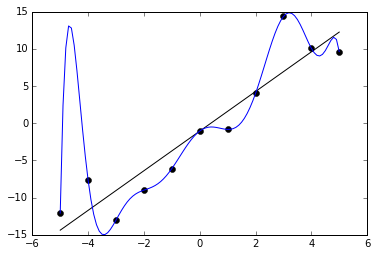
An example of this can be seen in the below graph. We are given 11 data points in black, and two functions are trained to fit it. One is a straight line, which roughly captures the data. The other is a very curvy line, which perfectly captures the data with no error. The latter may at first seem like the better fit because it has less (indeed, zero) error on the training data. But it probably does not really capture the underlying distribution very well and would have poor performance on unknown points.
How can we avoid overfitting? The simplest solution is to split our dataset into a training set and a test set. The training set is used for the optimization procedure we described above, but we evaluate the accuracy of our model by forwarding the test set to the trained model and measuring its accuracy. Because the test set is held out from training, this prevents the model from “cheating,” i.e. memorizing the samples it will be quizzed on later. During training, we can monitor the accuracy of the model on the training set and test set. The longer we train, the more likely our training accuracy is to go higher and higher, but at some point, it is likely the test set will stop improving. This is a cue to stop training at that point. We should generally expect that training accuracy is higher than test accuracy, but if it is much higher, that is a clue that we have overfit.
Cross-validation and hyperparameter selection
The procedure above is a good start to combat overfitting, but it turns out to be not enough. There remain a number of crucial decisions to make before optimization begins. What model architecture should we use? How many layers and hidden units should there be? How should we set the learning rate and other hyperparameters? We could simply try different settings, and pick the one that has the best performance on the test set. But the problem is we risk setting the hyperparameters to be those values which optimize only that particular test set, rather than an arbitrary or unknown one. This would again mean that we are overfitting.
The solution to this is to partition the data into three sets rather than two: a training set, a validation set, and a test set. Typically you will see splits where the training set accounts for 70 or 80% of the full data, and the test and validation are equally split among the rest. Now, you train on the training set, and evaluate on the validation set in order to find the optimal hyperparameters and know when to stop training (typically when validation set accuracy stops improving). Sometimes, cross-fold validation is preferred; in this type of setup, the training and validation set is split into some number (e.g. 10) equally-sized partitions, and each partition takes turns being the validation set. Other times, one validation set is used persistently. After validation, the final evaluation is carried out on the test data, which has been held out the whole time leading up to the end.
Recently, a number of researchers have even begun devising ways of learning architectures and hyperparameters within the training process itself. Researchers at Google Brain call this AutoML. Such methods hold great potential in automating those tedious components of machine learning which still require human intervention, and perhaps point to a future when someone will need only to define a problem and provide a dataset in order to do machine learning.
Regularization
Regularization refers to imposing constraints on our neural network in order to prevent overfitting or otherwise discourage undesirable properties. One way overfitting occurs is when the magnitude of the weights grows too large; it is this property that allows the shape of the network output function to curve so wildly as to capture the underlying noise of a training set, as we saw in the above example.
One way to regularize is to modify our objective function by adding an additional term which penalizes large weights. Denoting our neural network as \(f\), recall that the loss function we are optimizing is the mean squared error:
\[J = \frac{1}{n} \sum_i{(y_i - f(x_i))^2}\]We can penalize large weights by appending our loss function with the L2-regularization term, denoted here as $R(f)$:
\[R(f) = \frac{1}{2} \lambda \sum{w^2}\]This term is simply the sum of the squares of all of the weights, multiplied by a new hyperparameter $\lambda$ which controls the overall magnitude (and therefore influence) of the regularization term. The $\frac{1}{2}$ multiplier is simply used for convenience when taking its derivative. Adding it to our original loss function, we now have:
\[J = \frac{1}{n} \sum_i{(y_i - f(x_i))^2} + R(f)\]The effect of this regularization term is is that we help gradient descent find a parameterization which does not accumulate large weights and have such wild swings as we saw above.
Other regularization terms exist, including L1-distance or the “Manhattan distance.” Each of these have slightly different properties but have approximately the same effect.
Dropout
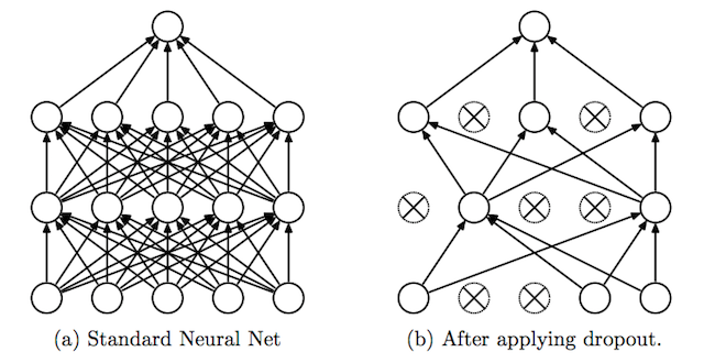
Dropout is a clever technique for regularization, which was only introduced by Nitish Srivastava et al in 2014. During training, when dropout is applied to a layer, some percentage of its neurons (a hyperparameter, with common values being between 20 and 50%) are randomly deactivated or “dropped out,” along with their connections. Which neurons are dropped out are constantly shuffled randomly during training. The effect of this is to reduce the network’s tendency to come to over-depend on some neurons, since it can’t rely on them being available all the time. This forces the network to learn a more balanced representation, and helps combat overfitting. It is depicted below, from its original publication.
Another exotic method for regularization is adding a bit of noise to the inputs. Still many others have been proposed with varying levels of success, but will not be covered in-depth here.
Backpropagation
At this point, we’ve introduced the gradient descent algorithm for parameterizing neural networks, along with a number of flavored alternatives including adaptive and momentum-based methods. Regardless of the exact variant chosen, all of them need to compute the gradient of the loss function with respect to the weights and biases of the network. This is no easy task. To see why, let’s think about how we might go about doing this.
Recall that our weight update formula in standard gradient descent is given by the following:
\[W_{t} := W_{t} - \alpha \nabla J(W_{t})\]$\nabla J(W_{t})$ is the gradient of the loss, and must be computed in some form across all of the gradient descent varieties we surveyed. Recall that the gradient is a vector which contains each of the individual partial derivatives of the cost function with respect to each parameter, and is given by the following ($t$ is omitted for brevity).
\[\nabla J(W) = \Biggl(\frac{\partial J}{\partial w_1}, \frac{\partial J}{\partial w_2}, \cdots, \frac{\partial J}{\partial w_N} \Biggr)\]How can we calculate each $\frac{\partial J}{\partial w_i}$? The most obvious way to do this would be to compute it with the equation for a derivative from ordinary calculus:
\[\frac{\partial J}{\partial w_i} \approx \frac{J(W + \epsilon e_i) - J(W)}{\epsilon}\]Where $e_i$ is a one-hot vector (all zeros except 1 at index $i$) and $\epsilon$ is a some very small number. Technically this will work, but it presents us with a major problem: speed. To get a single element of the gradient, it’s necessary to calculate the the loss function at both $W + \epsilon e_i$ and $W$. For $W$ it’s only necessary to do this once, but we need $J(W + \epsilon e_i)$ for every single weight $w_i$. Typical deep neural nets have millions or even hundreds of millions of weights. This would entail doing millions of forward passes, each of which has millions of operations, just to do a single weight update. This is totally impractical for training neural nets.
So how do we do it? In fact, until the development of backpropagation, this was a major impediment to training neural networks. The question of who invented backpropagation (“backprop” for short) is a contentious issue, and it seems that a number of people have re-invented it at different times throughout history, or stumbled upon similar concepts applied to different problems. Although largely associated with neural networks, backprop can be used on any problem that involves calculating a gradient on a continuously differentiable multivariate function, and as such, its development was somewhat parallel to the development of neural networks in general. In 2014, Jürgen Schmidhuber compiled a review of the relevant work that went into developing backprop.
Backpropagation was first applied to the task of optimizing neural networks by gradient descent in a landmark paper in 1986 by David Rumelhart, Geoffrey Hinton, and Ronald J. Williams. Subsequent work was done in the 80s and 90s by Yann LeCun, who first applied it to convolutional networks. The success of neural networks was largely enabled by their efforts along with their teams.
A full explanation of how backpropagation works is beyond the scope of this book. Instead, this paragraph will offer a basic high-level view of what backprop gives us, and defer a more technical explanation of it to a number of sources for further reading. The basic idea is that backprop makes it possible to compute all the elements of the gradient in a single forward and backward pass through the network, rather than having to do one forward pass for every single parameter, as we’d have to using the naive approach. This is enabled by utilizing the chain rule in calculus, which lets us decompose a derivative as a product of its individual functional parts. By keeping track of the differences in a forward pass along every connection and storing them, we can calculate the gradient by taking the loss term found at the end of the forward pass, and “propagating the error backwards” through each of the layers. This makes a backward pass take roughly the same amount of work as a forwards pass. This dramatically speeds up training and makes doing gradient descent on deep neural networks a feasible problem.
For more in-depth technical explanations of how backprop is derived, see the following links for further reading.
Descending the mountain
If you’ve made it this far into the article, then by now the analogy of the mountain climber put forth in the beginning of this chapter should be beginning to make sense to you. If that’s the case, congratulations: you appreciate the art and science of how neural networks are trained to a sufficient enough degree that actual scientific research into the topic should seem much more approachable. As the years have gone on, many scientists have proposed various and exotic extensions to backpropagation. Others, including Geoffrey Hinton himself, have suggested that machine learning must move on from backpropagation and start over. But as of the writing of this book, gradient descent via backpropagation continues to be the dominant paradigm for training neural networks and most other machine learning models, and looks to be set to continue on that path for the foreseeable future.
In the next few chapters of the book, we are going to start to look at more advanced topics. We will introduce Convolutional neural networks in the next chapter, as well as their numerous applications, especially toward art and other creative purposes that are at the heart of this book.