This tutorial will guide you on how to use the pix2pix software for learning image transformation functions between parallel datasets of corresponding image pairs.
What does pix2pix do?
pix2pix is shorthand for an implementation of a generic image-to-image translation using conditional adversarial networks, originally introduced by Phillip Isola et al. Given a training set which contains pairs of related images (“A” and “B”), a pix2pix model learns how to convert an image of type “A” into an image of type “B”, or vice-versa. For example, suppose we have pairs of images, where A is a black & white image and B is an RGB-color version of A, e.g. the following:
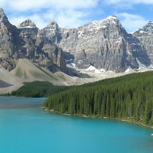
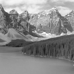
A pix2pix network could be trained on a training set of such corresponding pairs to learn how to make full-color from black & white images. Once a pix2pix network has been trained on such a dataset, it could then be used to color arbitrary black & white images. For example, below, we apply the learned colorization model on a black & white image from our test set, and generate a colored version of it. For comparison, we show the actual color image that it came with, to see how well the network is able to reconstruct the original color image (called the “target”).
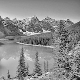

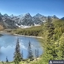
As we see above, the output is not identical to the input, but the network does a fairly decent job. We should expect that it will be able to color new, previously unseen black & white images to around the same accuracy.
Generalizing a bit
Many important image processing tasks can be framed as image to image translation tasks of this sort. Deblurring or denoising images can be framed in this way, and indeed there had been a great deal of past research in learning various specific image-to-image translation tasks like those and others. The nice thing about pix2pix is that it is generic; it does not require pre-defining the relationship between the two types of images. It makes no assumptions about the relationship and instead learns the objective during training, by comparing the defined inputs and outputs during training, and inferring the objective. This makes pix2pix highly flexible and adaptable to a wide variety of situations, including ones where it is not easy to verbally or explicitly define the task we want to model.
We get a good sense of this by considering a more complicated example, that of the CMP facades dataset which pix2pix has a download link for. Let’s look at a small sample of images from the facades dataset.
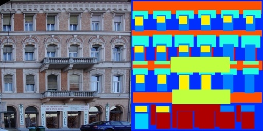
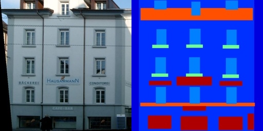
We have on one side photographs of building facades, and on the other side, their corresponding label maps which have been hand-labeled by human beings. The label maps are color-coded according to the object it’s representing, i.e. walls, windows, and doors. We can train pix2pix to generate the facade pictures from the label maps. If we do that, we can then attempt to generate an output from a test input, and compare the output to the original target image in the test dataset.
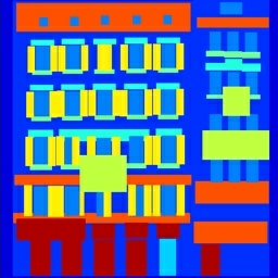
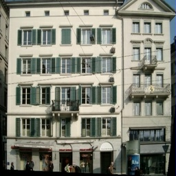
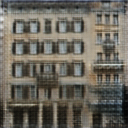
The output has numerous features that are different from the target, and has a somewhat different color, and is especially guessing in the regions where the labels are sparse. But it gets most of the main architectural features in the right place. This leads us to believe that we can mock up whole new label maps and create realistic looking facades from them! This could be very useful for an architect; they can sketch a design for a building and then quickly prototype textures for it (perhaps choosing from several dozen since they are so easy to produce).
Of course, we could have trained the network in the other direction as well; train it to generate the label maps from the real images. This can be very useful as well; suppose you are in charge of a startup which is generating special types of label maps from satellite images. This provides a way to do it quickly and cheaply.
Another important quality of pix2pix is that it requires a relatively small number of examples – for a low-complexity task, perhaps only 100-200 samples, and usually less than 1000, in contrast to networks which often requires tens or even hundreds of thousands of samples. The downside is that the model loses some generality, perhaps overfitting to the training samples, and thus can feel a bit repetitive or patchy. Still, those practical advantages make it extremely easy to deploy for a wide variety of images, enabling rapid experimentation. Since we aren’t burdened with having to collect tens of thousands of examples, we may be able to create our own datasets with relatively little overhead.
Getting creative with it
The beauty about a trained pix2pix network is that it will generate an output from any arbitrary input. So far, we’ve looked at examples for which we already knew the correct output (the target), so that we could visually compare them. But the network will take in just about anything once it’s trained, giving us some space to be creative. Let’s look at some examples.
Sketches to objects
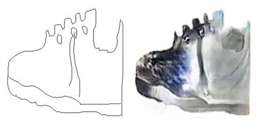
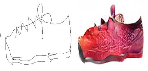
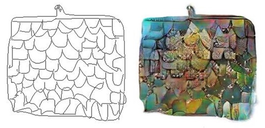
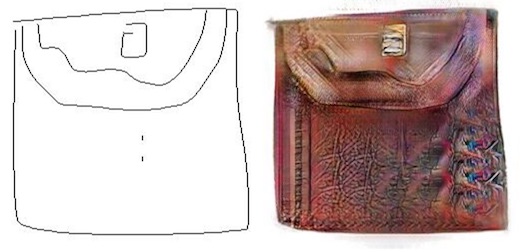
The original pix2pix software came with a number of “sketch to object” datasets. These were usually a number of images of some kind of object (say shoes) along with its edge map (the “sketch”) which can be cheaply extracted from the image using standard image-processing techniques (like Canny edge detection in OpenCV). By training a pix2pix network to convert the sketch into the image, we are then able to use the model to convert a new unseen sketch into an image of the object type.
Here are some samples of sketches being turned into shoes.
As well as sketches being turned into handbags.
Sketch2Cat
Christopher Hesse made an excellent online demo demonstrating the “sketch to something” technique by training a pix2pix model to generate images of cats from their edge maps.
Additionally, he wrote a very good description of what pix2pix does, as well as the tensorflow implementation of pix2pix that the practical part of this guide will use later.
Image-to-Image Tensorflow Demo https://t.co/KUdUPA1IXx pic.twitter.com/1QQPyGlo1F
— Christopher Hesse (@christophrhesse) February 19, 2017
Invisible Cities
One collaborative work (of which the writer of this guide was involved in) was a project called “Invisible Cities”, made during an ml4a workshop at OpenDot Lab in Milan, Italy. The project was completed in the same week that the original paper and repository was released, demonstrating how quickly one can create an applied work from it.
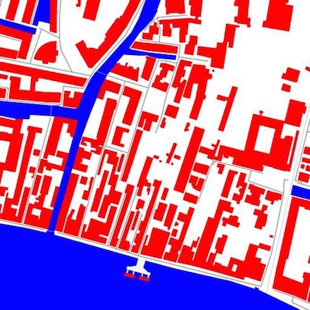
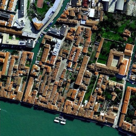
In Invisible Cities, a collection of map tiles and their corrsponding satellite images from multiple cities were downloaded from the MapBox API. A pix2pix model was trained to convert the map tiles into the satellite images.
Below is an example pair from one dataset of maps from Venice, Italy.
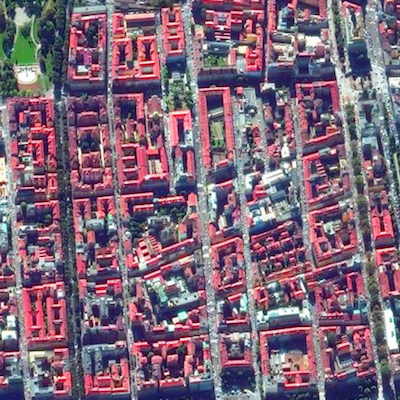
After training the Venice model, we take a map tile from a different city, Milan, Italy, and run it through the Venice pix2pix generator.
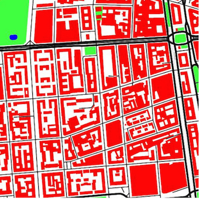
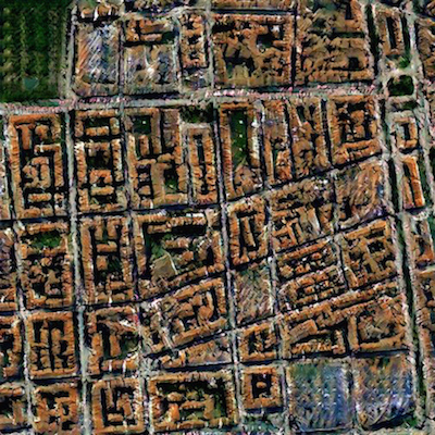
We can also make fake inputs entirely by just drawing them by hand, like the following:
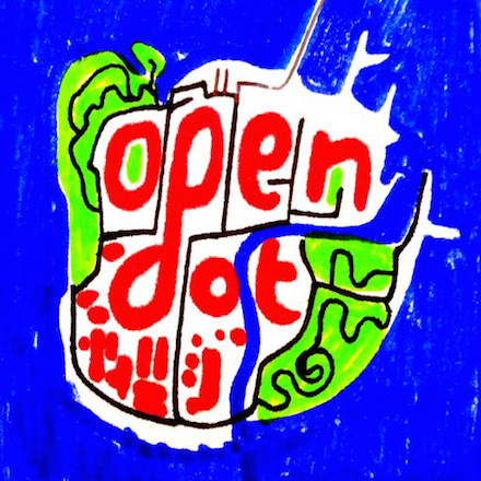
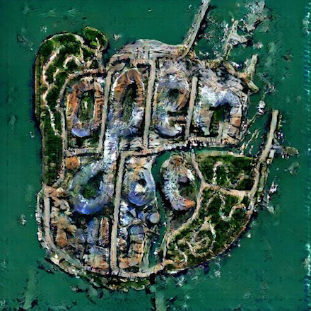
More examples can be found in the gallery of the main project page.
Neural City
In Neural City, Jaspaer van Loenen trained pix2pix on Google streetview images to convert depth maps into street view photos.
First try at generating streetview-like cityscapes #deeplearning #pix2pix pic.twitter.com/SP3WiAHL0M
— Jasper van Loenen (@JaspervanLoenen) March 14, 2017
— Jasper van Loenen (@JaspervanLoenen) April 5, 2017
FaceTracker -> Face
Another clever dataset to work with are images of faces matched to their detected facetracker landmarks. By training pix2pix to convert the facetracker representation to the original images of faces, you can generate faces from an arbitrary set of landmarks. See the following by Mario Klingemann who trained pix2pix to generate face sketches trained on sketches found in the dataset from the British Library.
Generating faces from a sketch. I trained a pix2pix net on 1500 #bldigital faces. Left input, right output. pic.twitter.com/IPi9VmI2Li
— Mario Klingemann (@quasimondo) January 30, 2017
Another experiment from Mario was training the generator on YouTube videos of Francoise Hardy, then tracking the face of KellyAnne Conway while she explained “alternative facts,” and generating images of Francoise Hardy from those found landmarks, effectivly making Francoise Hardy pantomime the facial gestures of KellyAnne Conway.
Riffing on this technique, I made a webcam-enabled pix2pix trained on pictures of Donald Trump’s face giving a speech. The real-time application was run live for a workshop.
my new meat puppet. running #pix2pix live on a webcam pic.twitter.com/wVc5DuCXeG
— Gene Kogan (@genekogan) April 28, 2017
Person-to-person pix2pix
Brannon Dorsey trained pix2pix on image pairs of Ray Kurzweil giving a talk and himself mimicking Kurzweil’s gestures. The result let him create generative versions of himself in the pose of Ray Kurzweil on stage.
Full person-to-person image translation with machine learning! Applying #pix2pix to video @branger_briz @phillip_isola @genekogan @kaihuchen pic.twitter.com/oFrzj1qcqt
— Brannon Dorsey (@brannondorsey) December 6, 2016
Live drawing interfaces
In addition to the “sketch2cat” interface mentioned above, other works have made use of pix2pix’s capacity to generate in real-time.
Bertrand Gondouin trained pix2pix to turn sketches of pokemon into actual pokemons in a live drawing interface.
Sketches done using a graphics tablet, colored by a a real-time neural network trained unsupervised on #Pokemon pictures (x2) #pix2pix, #AI pic.twitter.com/MIW8HfO8KU
— Bertrand Gondouin (@bgondouin) January 9, 2017
As did Memo Akten, training a network to convert Canny edge detections from a webcam to generate images trained from a dataset containing the collections of 150 museums. Memo also released his code for running the webcam demo.
...#GAN trained on art collections of 150 museums watching me draw... pic.twitter.com/yArZLauzSI
— Memo Akten (@memotv) April 29, 2017
As a follow-up to Invisible Cities, I made a drawing interface with p5.js and a node-based server-client setup (much like sketch2cat) and released the code as well.
Using pix2pix
The following is a tutorial for how to use the tensorflow version of pix2pix. If you wish to, you can also use the original torch-based version or a newer pytorch version which also contains a CycleGAN implementation in it as well. Although these instructions are for the tensorflow version, they should be fairly relevant to the others with just minor modifications in syntax. You should be able to use any of the versions and get similar results.
In using pix2pix, there are two modes. The first is training a model from a dataset of known samples, and the second is testing the model by generating new transformations from previously unseen samples.
Training pix2pix means creating, learning the parameters for, and saving the neural network which will convert an image of type X into an image of type Y. In most of the examples that we talked about, we assumed Y to be some “real” image of dense content and X to be a symbolic representation of it. An example of this would be converting images of lines into satellite photographs. This is useful because it allows us to generate sophisticated and detailed imagery from quick and minimal representations. The reverse is possible as well; to train a network to convert the real imagery into its corresponding symbolic form. This can be useful for many practical tasks; for example automatically finding and labeling roads and infrastructure in satellite images.
Once a model has been generated, we use testing mode to output new samples. For example, if we trained X->Y where X is a symbolic form and Y is the real form, then we make generative Y images from previously unseen X symbolic images.
Installation
In order to run the software on your machine, you need to have an NVIDIA GPU which is supported by CUDA. Here is a list of supported devices. At least 2GB of VRAM are recommended, although realistically, with less than say 4GB, you may have to produce smaller-sized samples. If you have an older laptop, consider using a cloud-based platform instead (todo: make a guide about cloud platforms).
Install CUDA
Once you have successfully run the installer for CUDA, you can find it on your system in the following locations:
- Mac/Linux: /usr/local/cuda/
- Windows: C:\Program Files\NVIDIA GPU Computing Toolkit\CUDA\v8.0
In order for your system to find CUDA, it has to be located in your PATH variables, and in LD_LIBRARY_PATH for Mac/Linux. The installer should do this automatically.
Install cuDNN
cuDNN is an add-on for CUDA which specifically implements operations for deep neural nets. It is not required to run Tensorflow but is highly recommended, as it makes many of the programs much more resource-efficient, and is probably required for pix2pix.
You have to register first with NVIDIA (easy) to get access to the download. You should download the latest version for your platform unless you have an older version of CUDA. At time of this writing, cuDNN 5.1 works with CUDA 8.0+, although cuDNN 6.0+ should work as well.
Once you’ve download cuDNN, you will see it contains several files in folders called “include”, “lib” or “lib64”, and “bin” (if on windows). Copy these files into those same folders inside of where you have CUDA installed (see step 1)
Install tensorflow
Follow tensorflow’s instructions for installation for your system. In most cases this can be done with pip.
Install pix2pix-tensorflow
Clone or download the above library. It is possible to do all of this with the original torch-based pix2pix (in which case you have to install torch instead of tensorflow for step 3. These instructions will assume the tensorflow version.
Training pix2pix
First we need to prepare our dataset. This means creating a folder of images, each of which contain an X/Y pair. The X and Y image each occupy half of the full image in the set. Thus they are the same size. It does not matter which order they are placed into, as you will define the direction in the training command (just remember which way because you need to be consistent).
Additionally, by default the images are assumed to be square (if they are not, they will be squashed into square input and output pairs). It is possible to use rectangular images by setting the aspect_ratio argument (see the optional arguments below for more info).
Then we need to open up a terminal or command prompt (possibly in administrator mode or using sudo if on linux/mac), navigate (cd) to the directory which contains pix2pix-tensorflow, and run the following command:
python pix2pix.py --mode train --input_dir /Users/Gene/myImages/ --output_dir /Users/Gene/myModel --which_direction AtoB --max_epochs 200
replacing the arguments for your own task. An explanation of the arguments:
--mode : this must be “train” for training mode. In testing mode, we will use “test” instead.
--input_dir : directory from which to get the training images
--output_dir : directory to save the model (aka checkpoint)
--which_direction : AtoB means train the model such that the left half of your training images is the input and the right half is the output (generated). BtoA is the reverse.
--max_epochs : number of epochs (iterations) to train, i.e. how many times to each image in your training set is passed through the network in training. In practice, more is usually better, but pix2pix may stop learning after a small number of epochs, in which case it takes longer than you need. It is also sometimes possible to train it too much, as if to overcook it, and get distorted generations. The loss function does not necessarily correspond well to quality of images generated (although there is recent research which does create a better equivalency between them).
Note also that the order in which parameters are written in the command does not actually matter. Additionally, there are optional parameters which may be useful:
--checkpoint : a previous checkpoint to start from; it must be specified as the path which contains that model (so it is equivalent to –output_dir). Initially you won’t have one but if your training is ever interrupted prematurely, or you wish to train for longer, you can initialize from a previous checkpoint instead of starting from scratch. This can be useful for running for a while and checking to see quality, and then resuming training for longer if you are unsatisfied.
--aspect_ratio : this is 1 by default (square), but can be used if your images have a different aspect ratio. If for example your images are 450x300 (width is 450), then you can use an aspect_ratio 1.5.
--output_filetype : png or jpg
There are more advanced options, which you can see in the arguments list in pix2pix.py. The adventurous may wish to experiment with these as well.
Unfortunately, pix2pix-tensorflow does not currently allow you to change the actual size of the produced samples and is hardcoded to have a height of 256px. Simply changing it in pix2pix.py will result in a shape mismatch. If you wish to generate bigger samples, you can do so using the original torch-based pix2pix which does have it as a command line parameter, or more adventurously adapt the tensorflow code to arbitrarily sized samples. This will require changing the architecture of the network slightly, perhaps as a function of a –sample_height parameter, which is a good exercise left to the intrepid artist.
In practice, trying to generate larger samples, say 512px does not always lead to improved results, and may instead look not much better than an upsampled version of the 256px versions, at the cost of requiring significantly more system resources/memory and taking longer to finish training. This will definitely be true if your original images are smaller than the desired size because subpixel details are not available in the training data, but even if your data is sized sufficiently, it may still occur. Worth trying out, but your results may vary.
Once you run the command, it will begin training, updating the progress periodically and will consume most or all of your system’s resources so it’s often worth running overnight.
Testing or generating images
The second operation of pix2pix is generating new samples (called “test” mode). If you trained AtoB for example, it means providing new images of A and getting out hallucinated versions of it in B style.
In pix2pix, testing mode is still setup to take image pairs like in training mode, where there is an X and a Y. This is because a useful thing to do is to hold out a test or validation set of images from training, then generate from those so you can compare the constructed Y to the known Y, as a way to visually evaluate the data. pix2pix helpfully creates an HTML page with a row for each sample containing the input, the output (constructed Y) and the target (known/original Y). Several of the downloadable datasets (e.g. facades) are packaged this way. In our case, since we may not have the corresponding Y (after all, that’s the whole point!) a quick workaround for this problem is to simply take each X, and convert into an image twice the width where one half is the image to use as the input (X) and the other is some blank decoy image. Make sure you are consistent with how it was trained; if you trained –which_direction AtoB, the blank image is on the right, and BtoA it is on the left. If the generated html page shows the decoy as the “input” and the output is the nondescript “Rothko-like” image, then you accidentally put them in the wrong order.
Once your testing data has been prepared, run the following command (again from the root folder of pix2pix-tensorflow):
python pix2pix.py --mode test --input_dir /Users/Gene/myImages/ --output_dir /Users/Gene/myGeneratedImages --checkpoint /Users/Gene/myModel
An explanation of the arguments:
--mode : this must be “test” for testing mode.
--input_dir : directory from which to get the images to generate
--output_dir : directory to save the generated images and index page
--checkpoint : directory which contains the trained model to use. In most cases, this should simply be the same as the –output_dir argument in the original training command.
todo: example images through training and testing process
todo: make a CycleGAN guide